Syllabus. Here are the math/stat department policies, university policies and the COVID policies that are also part of the syllabus. Here is the Jacks are Back website that has the latest info about NAU policies regarding COVID.
Office hours: in my office, AMB 110, unless otherwise noted. Please wear a mask for office hours.
M: 10:20-11:30
Tu: 12:25-12:45 in AMB 148 (between my 2 sections of MAT 239, but 238 students can come too)
W: 10:20-11:30
Th: 12:25-12:45 in AMB 148, and 2:20-3:00 in my office
F: 10:20-11:30
Please feel free to contact me any time via e-mail with any questions about the math, or with any feedback about the class.
Recommended text:
Calculus Early Transcendentals, 3rd Edition, by Rogawski and Adams. You can buy a used copy online
for less than $15, or rent for less than that.
A free online textbook is
Calculus: early transcendentals from Whitman College.
The NAU math/stat department is using Whitman as the textbook for Calc 1 this semester, and next semester it will
be used for Calc 1 and 2, and the next semester for Calc 1, 2, and 3.
An alternative free textbook is OpenStax Calc 3.
You can also consult
Paul Dawkins' Calc 3 Notes.
Paul's notes on Vectors are at the end of his Calc 2 notes.
Here is an Introduction to WeBWorK.
You probably won't need this if you have used WeBWorK in a previous class.
NOTE: You login name is your LOUIE account (e.g. jws8).
Your password is same one you always use with this login name.
For 2-D plotting, I like Desmos Graphing Calculator.
Here is a link to CalcPlot3D.
Mathematica is available at the CEFNS computer labs on north campus, and at open
labs in the Geology, Math, Chemistry, and SLF buildings. (But the Engineering School does not really embrace Mathematica much.) It is also available on the NAU Microsoft Virtual Desktop http://apps.nau.edu.
You can even get a copy installed on your machine. See Mathematica Licenses for Students.
General information is available at the ITS article: Mathematica at NAU.
This is a great webcast introducing you to
Mathematica.
You can get extra credit for our course from points earned in the
Problem of the Week.
You can get up to 3 class points per week.
FAMUS
(Friday Afternoon Undergraduate Math Seminar): Fridays at 3 pm in AMB 164.
NAU offers free help in this class through the Math Achievement Program and the Academic Success Center.
Final Exam Review Session for Calc 3: Wednesday, Dec. 1, from 6-7pm in the MAP room (AMB 137). A recording will be available.
Review of Chapters 16 and 17
Graphs of vector fields with constant divergence and curl.
Here is the Mathematica Notebook, VectorFieldDivCurl.nb that made that pdf.
Feynman Lectures on Physics
The two lectures linked to below give an overview of our Chapters 16 and 17. I recommend looking at these if you are interested in physics.
(But don't try to understand everything! Just let Feynman's genius wash over you.) Volume III of the Feynman Lectures on Physics is mostly about Electricity and Magnetism.
Differential Calculus of Vector Fields (Volume III, Chapter 2)
Vector Integral Calculus (Volume III, Chapter 3)
The equations of Electrostatics for the electric field
\(\mathbf{E}(x,y,z)\) are \(\nabla \cdot \mathbf{E} = \frac{1}{\epsilon_0} \rho, \ \nabla \times \mathbf{E} = \mathbf{0}\), where \(\rho\) is the charge density.
The equations of Magnetostatics for the magnetic field
\(\mathbf{B}(x,y,z)\) are \(\nabla \cdot \mathbf{B} = 0, \ \nabla \times \mathbf{B} = \mu_0 \mathbf{J}\), where \( \mathbf{J}\) is the current density.
The equations get more complicated, and they describe light, when you add time dependence.
Section 17.3: Divergence Theorem
Paul's notes
Justification of the Divergence theorem, pictures of the white board: Part 1.
We can approximate any shape with minecraft blocks, and then do Part 2
Videos
Divergence Theorem 1
Divergence Theorem 1
Divergence Theorem to Evaluate Flux Integral (Spherical Coordinates)
3D divergence theorem intuition
Flux and the divergence theorem
Divergence Theorem explanation
Section 17.2: Stokes’ Theorem
Paul's notes
Justification of Stokes’ Theorem, picture of the white board
StokesTheorem.pdf.
Note: That pdf should mention that the curve \(\mathcal C\) is the boundary of
the surface \(\mathcal S\), that is, \(\mathcal C = \partial \mathcal S\).
Videos
Stokes’ Theorem 1
Stokes’ Theorem 2
Stokes’ theorem intuition
Stokes’ Theorem
Section 17.1: Green’s Theorem
Paul's notes
Justification of Green’s theorem, pictures of the white board: Part 1, Part 2.
Videos
Green's Theorem
Green's Theorem 2
Green's Theorem to find Area Enclosed by Curve
Area using Line Integrals
Section 16.4 and 16.5: Surface Integrals
Paul's notes on Surface Integrals of
scalar fields
and
vector fields
Videos of surface integrals of scalar fields
Parameterized Surfaces
Area of a Parameterized Surface
Surface Integrals
Surface Integrals 2
Surface Integral triangular region
Videos of surface integrals of vector fields
Surface Integral of Vector Field
Surface Integral of Vector Field 2
Surface Integral Using Polar Coordinates
Section 16.3: Conservative Vector Fields
Paul's notes on
Fundamental Theorem of Line Integrals
and
Conservative Vector Fields
Videos
Fundamental Theorem of Line Integrals
Closed curve line integrals of conservative vector fields
Conservative Vector Fields
Fundamental theorem of line integrals
Section 16.2: Line Integrals
Paul's notes for
Scalar
and
Vector
Line Integrals.
Videos of Scalar Line Integrals (Curve integrals of scalar fields)
Line integral 2D
Line integral 3D
Mass of wire
Videos of Vector Line Integrals (Curve integrals of vector fields)
Parametrization piecewise
Work
Differential form
Line segment
Section 16.1: Vector Fields
Paul's notes
There are tons of applications for vector fields!
Here is a wind map of the USA. Here is the wikipedia page for
Maxwell's Equations which describe electric and magnetic fields (E and B).
Here is a picture of a
vortex behind an airplane wing.
Here is a GeoGebra app to plot a 2D vector field.
Here is a notebook to
plot a 2-dimensional vector field with
Mathematica. You can also search the web for programs.
Most vector field plotters scale the vectors.
Videos
Two-dimensional vector fields
Divergence and curl (definitely watch this)
Divergence
Sign of the Divergence
Curl
Curl intuition
Curl nuance
Three-dimensional vector fields
Divergence 1
Divergence 2
Curl 1
Curl 2
Curl 3
Section 15.6: Changes of Variables
Paul' notes on Change of Variables
(Paul's does not have a stand-alone section on applications.)
Here is my Mathematica File showing examples of a Change of Variables.
Videos
Change of variables
Triangle
Parallelogram
Jacobian 2x2
Jacobian 2x2
Jacobian 3x3
Section 15.5: Applications
Videos
Mass 3D
Center of mass of triangle
Center of mass of cube
Center of mass paraboloid
Section 15.4: Double integrals in Polar Coordinates, Triple integrals in Cylindrical or Spherical Coordinates
Paul's notes about polar,
cylindrical, and
spherical coordinates.
Videos
my video about
Integrals in spherical and cylindrical coordinates
Changing to polar
Changing to cylindrical
Volume of sphere
Spherical coordinates
Section 15.3: Triple Integrals
Paul's notes
Videos
Triple integral
Tetrahedron
Cylinder
Volume
Different order of integration
Section 15.2: Double Integrals over Non-Rectangular Regions
Paul's notes
Videos
Triangular region
More general region
More general region
Both order of integration
Change order of integration
Change order of integration
Section 15.1: Double Integrals over Rectangles
Paul's notes
and
more of Paul's notes
Videos
Double integrals
Approximate volume from table of values
Approximate double integral from contour plot
Fubini
Double integral on rectangular region
Average value over rectangular region
Section 14.8: Lagrange Multipliers
Paul's notes
Help on Problem 4.
With my three data points, (1,0), (5,5), and (7,10) I can a perfect fit \(y = a x^2 + b\) that has \(S(a,b) = 0\),
as seen in this desmos graph.
But that most random numbers do not allow a perfect fit like this.
Videos
Lagrange Multipliers two variables one constraint
Lagrange Multipliers three variables one constraint
Global extrema on disk
Lagrange Multipliers three variables two constraints
Section 14.7: Part 2: Local Extrema
Paul's notes
on relative extrema which is another word for local extrema.
Videos
Critical points, second derivative test
Local extrema
Local extrema
Minimum distance of point from plane
Minimum surface area of box
Maximum volume of box
Minimum cost of box
Distance between point and cone
Section 14.7: Part 1: Global Extrema
Paul's notes
on absolute extrema which is another word for global extrema.
Videos
Global extrema, rectangular domain
Global extrema, circular domain
Section 14.6: The Chain Rule.
Paul's notes
Figure showing the dependency diagram for Problem 4 on the webwork
Videos
Chain rule with partial derivatives from the Organic Chemistry tutor
The Multi-variable chain rule from Trefor Bazett
Section 14.5: The Gradient and Directional Derivatives.
Paul's notes on the directional derivative
and the
gradient
My web page on gradients.
Videos
My video on problem 6 in the WeBWorK
My video on problem 8 in the WeBWorK
Gradient
Directional Derivative
Directional Derivatives and the Gradient
Max rate of change
Directional Derivative in 3D calc plotter
Gradient in 3D calc plotter
Normal vector
Tangent plane example
Section 14.4: The Tangent Plane to the graph of \(f: \mathbb{R}^2 \to \mathbb{R}\)
Paul's notes
Videos
Local linearization
Tangent plane
Tangent plane (exponential)
Tangent plane (trigonometric)
14.3: Partial derivatives
Paul's notes have 3 sections:
Partial derivatives,
their interpretation, and
higher order partial derivatives
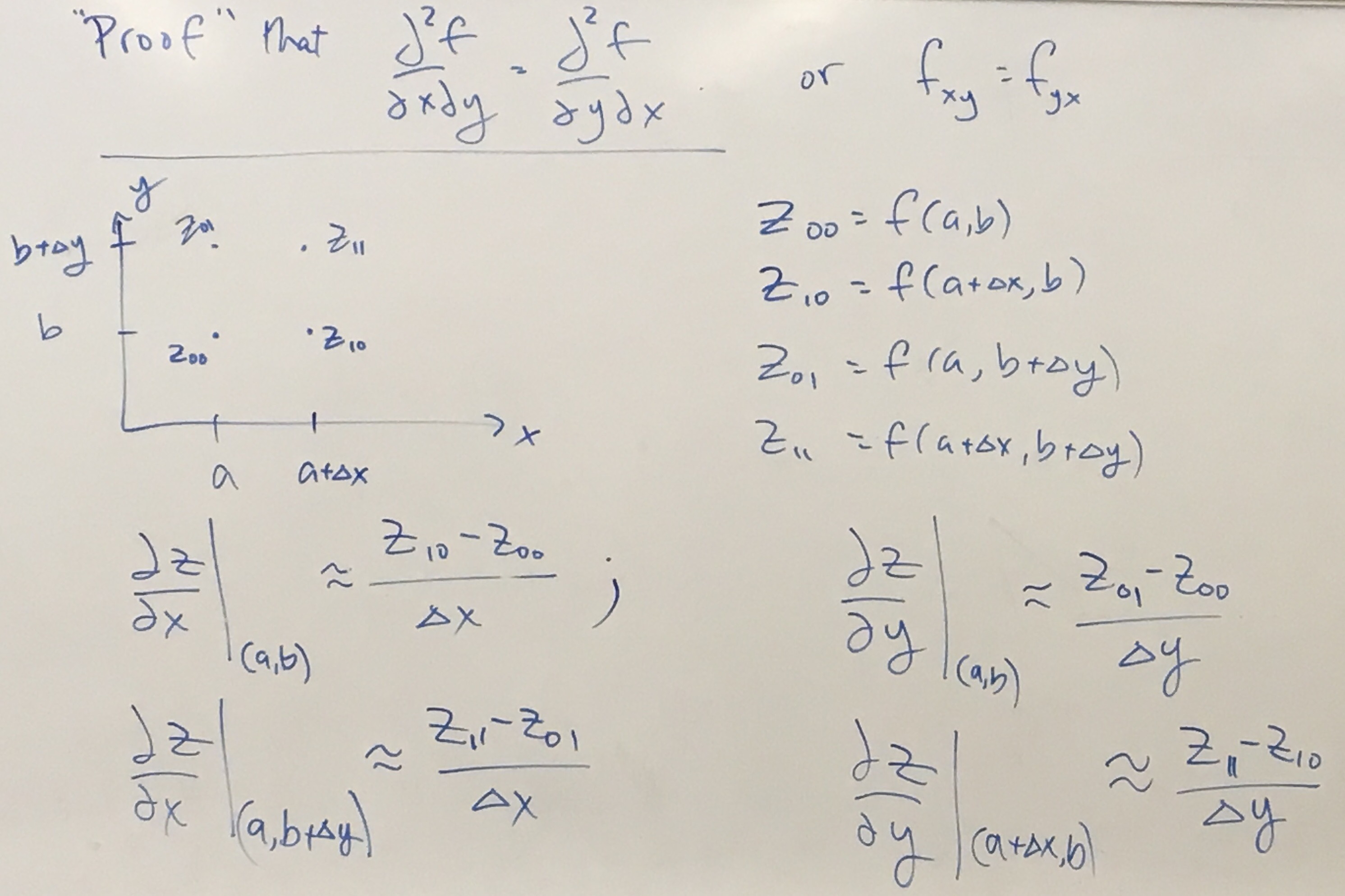
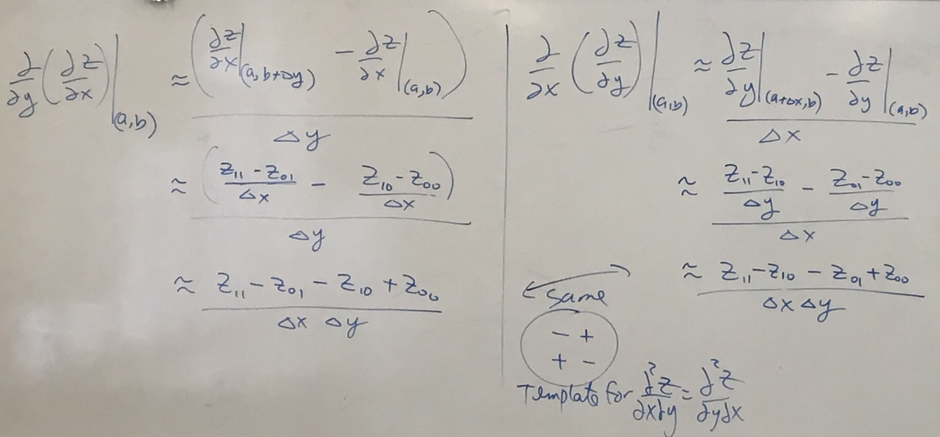
Here are pictures of a demonstration that mixed partial derivatives are equal:
page 1 and page 2.
Videos
Partial derivatives
Partial derivative example
Partial derivative from contour plot
Second partial derivatives
Second partial derivatives
Section 14.2: Limits of Real-Valued Functions of Two Variables
Paul's notes
Videos
Limits are...weird..for multi-variable functions
Limits of Functions of Two Variables
Example 1
Example 2
Example 3
Section 14.1: Real-Valued Functions of Several Variables
This Mathematica notebook shows the level surface in Set 14.1, problem 12.
You can see this in the computer lab in room 222 in the Math building, or any computer lab on campus with Mathematica.
See this site about Mathematica at NAU.
You can get Mathematica for your own computer!
I realize that not all of you can access mathematica, so here is a
pdf of the level surface in Set 14.1, problem 12.
Even though this is a static image, it is much easier to decipher than the figure in webwork.
See this site with a link to
Mathematica at NAU.
You can get Mathematica for your own computer!
Videos
Finding domain
Level curves, contour plot
Function value from contour plot
Increasing or decreasing from contour plot
Traces
Graph Two Variable Function with 3D Calc Plotter
Contour plot with 3D Calc Plotter
Midterm 1 will be in class on Monday, Sept. 20. There is a sample exam
on BbLearn.
Here is a link to a BbLearn video of a
review session
run by the Math Achievement program. Your browser needs to be using your LOUIE id.
Section 13.3 and 13.5: Speed, velocity, and acceleration
Paul's notes
Videos
Velocity, speed, direction, and acceleration
Velocity and Position from Acceleration
Section 13.2: Calculus of vector-valued functions
Paul's notes
Videos
Derivative of vector-valued functions
Properties
More properties
Equation of tangent line
Angle of two curves
Integration with Initial Conditions
Definite integral
Section 13.1: Vector-valued functions
Paul's notes
Here is the GeoGebra 3D calculator. It is an alternative
to the CalcPlot3D app.
Please send me any other
suggested apps.
Here is a Mathematica notebook, helix.nb,
that will plot a parameterized curve in \(\mathbb{R}^3\).
It is harder to use than some other programs, but the pictures are beautiful.
This Mathemtica notebook will Plot 2 Surfaces And 1 Curve.
Videos
Vector valued functions
Domain of a Vector Valued Function
space curves in 3D Calc Plotter
Curve of intersection of two surfaces
Curve of intersection of two surfaces
Vector Valued Function from a Rectangular Equation
Section 12.7: Cylindrical and Spherical Coordinates.
Here are Paul's notes on
polar,
cylindrical, and
spherical coordinates.
BEWARE! Paul lies to you. He writes the formula “\(\theta = \tan^{-1} (\frac y x )\)”,
which is wrong in two ways: It is false half the time,
and it uses the abominable notation “\(\tan^{-1}\)” instead of “\(\arctan\)”.
Remember, the best single formula we can write is
“\(\tan(\theta) = \frac y x\), provided \(x \neq 0\).”
To compute \(\theta\) you need to draw a darn picture!
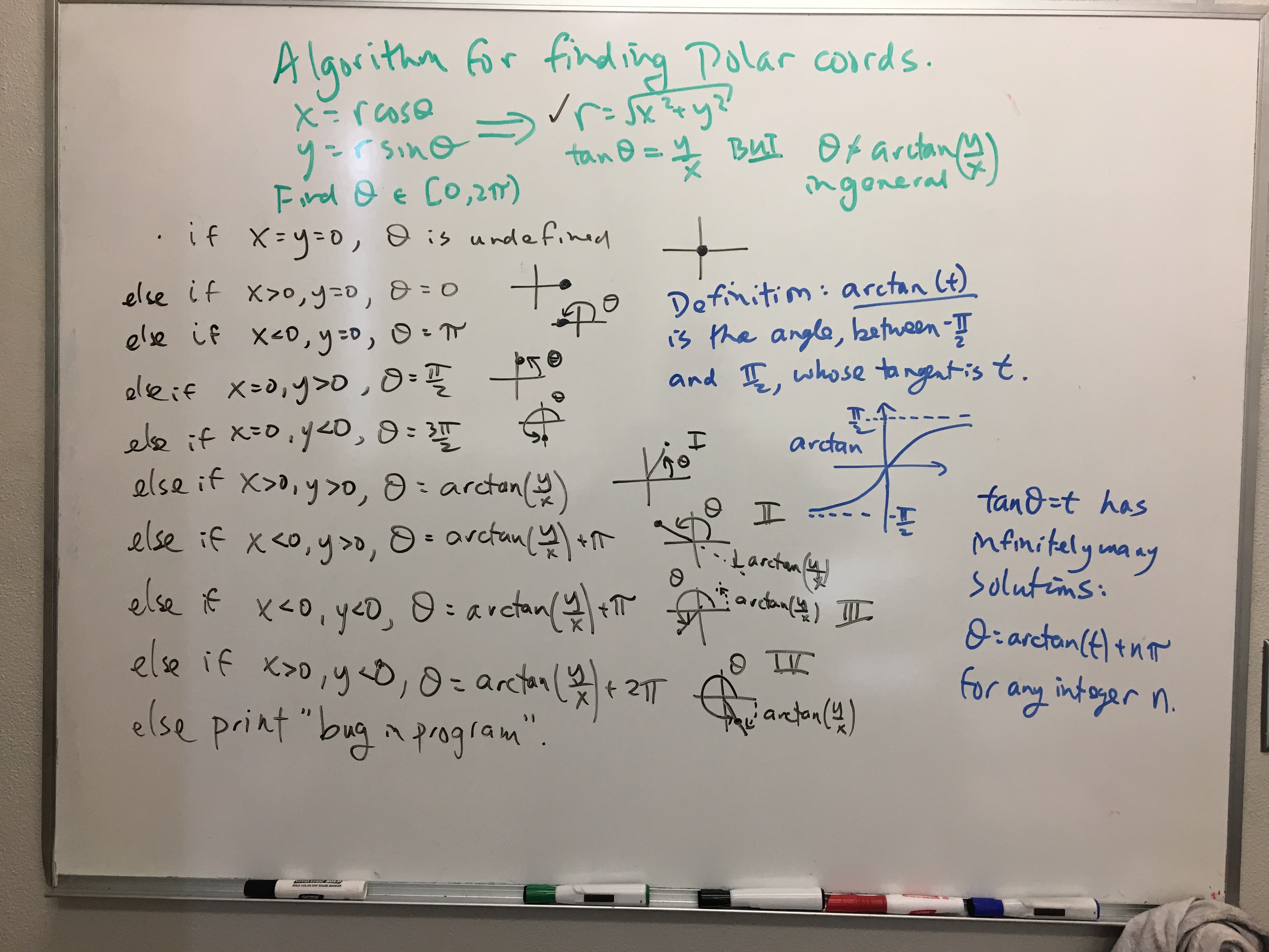
Here is a figure about how to compute theta in polar or cylindrical
or spherical coordinates using the picture you have drawn.
For those who prefer a formula,
I wrote this algorithm for finding \(\theta\).
Note that \(\arctan(y/x)\) is undefined if \(x = 0\), so those cases are handled first.
I don't intend you humans to follow this algorithm exactly: Just draw the #!#! picture.
Videos
Cylindrical Coordinates
Spherical Coordinates
Cartesian Coordinates to Spherical
Spherical Coordinates to Cartesian
Cartesian Coordinates to Cylindrical
Cylindrical Coordinates to Cartesian
Cylindrical Equations to Rectangular
Rectangular Equations to Cylindrical
Spherical Equations to Rectangular
Rectangular Equation to a Spherical
Spherical Equation to a Rectangular
Section 12.6: Quadratic Surfaces
Paul's notes
Videos
Cylindrical Surfaces
Quadric Surfaces
Ellipsoid
Elliptical Cone
Elliptical Paraboloid
Hyperbolic Paraboloid
Surfaces in 3D Calc Plotter.
This video talks about the CalcPlot3D
app.
Section 12.5: Planes in space
Paul's notes
Desmos graph for the line 3x + 2y = 7 in the plane, written as the line through (0, 3.5) with normal vector (3, 2).
Videos
Normal equation of plane
Point of Intersection of a Plane and a Line
Point of Intersection of a Plane and a Line
Intersection to two planes
Line through a point and perpendicular to a plane
Plane given with point and parallel plane
Plane given with three points
Plane given with three points
Plane given with point and orthogonal line
Angle between two planes
Distance between point and plane
Distance between parallel planes
Distance between line and point
Section 12.4: The Cross Product.
Paul's notes
Example: calculation of the cross product done in two ways.
This is my problem 6 on the WeBWorK. You only need to do it one way, but it's comforting that they
give the same answer.
Suggested videos on matrices
Multiplying matrices
2x2 determinant
3x3 determinant
Suggested videos on the cross product
Cross product
Cross product
Cross product example
Area of space triangle
Volume of parallelepiped
Section 12.3: The Dot Product.
Paul's notes
Suggested videos.
Dot product
Angle between vectors
Parallel and perpendicular components
Section 12.2: Vectors in \(\mathbb{R}^3\)
Paul's notes
Suggested videos.
Parametric equation of line in 3D
Parametric equation of line in 3D
Intersection of two lines
Section 12.1: Vectors
Paul's notes on
basics and
vector arithmetic.
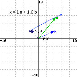
The answer to one version of WeBWorK problem 10 in set 12.1 is
x = a + 1.6 b. (So type 1 and 1.6 into the two blanks.)
This figure shows the vectors.
Here is a Mathemetica notebook to allow arbitrary linear combinations of
a and b.
Suggested videos.
Vector operations: Sum, scalar multiple, dot product
Length of a 3D vector
Unit vectors: Direction of a vector
Plotting points