Review of Chapters 16 and 17
Graphs of vector fields with constant divergence and curl.
Here is the Mathematica Notebook, VectorFieldDivCurl.nb that made that pdf.
Feynman Lectures on Physics
The two lectures linked to below give an overview of our Chapters 16 and 17. I recommend looking at these if you are interested in physics.
(But don't try to understand everything! Just let Feynman's genius wash over you.) Volume III of the Feynman Lectures on Physics is mostly about Electricity and Magnetism.
Differential Calculus of Vector Fields (Volume III, Chapter 2)
Vector Integral Calculus (Volume III, Chapter 3)
The equations of Electrostatics for the electric field
\(\mathbf{E}(x,y,z)\) are \(\nabla \cdot \mathbf{E} = \frac{1}{\epsilon_0} \rho, \ \nabla \times \mathbf{E} = \mathbf{0}\), where \(\rho\) is the charge density.
The equations of Magnetostatics for the magnetic field
\(\mathbf{B}(x,y,z)\) are \(\nabla \cdot \mathbf{B} = 0, \ \nabla \times \mathbf{B} = \mu_0 \mathbf{J}\), where \( \mathbf{J}\) is the current density.
The equations get more complicated, and they describe light, when you add time dependence.
Section 17.3: Divergence Theorem
Paul's notes
Justification of the Divergence theorem, pictures of the white board: Part 1.
We can approximate any shape with minecraft blocks, and then do Part 2
Videos
Divergence Theorem 1
Divergence Theorem 1
Divergence Theorem to Evaluate Flux Integral (Spherical Coordinates)
3D divergence theorem intuition
Flux and the divergence theorem
Divergence Theorem explanation
Section 17.2: Stokes’ Theorem
Paul's notes
Justification of Stokes’ Theorem, picture of the white board
StokesTheorem.pdf.
Note: That pdf should mention that the curve \(\mathcal C\) is the boundary of
the surface \(\mathcal S\), that is, \(\mathcal C = \partial \mathcal S\).
Videos
Stokes’ Theorem 1
Stokes’ Theorem 2
Stokes’ theorem intuition
Stokes’ Theorem
Section 17.1: Green’s Theorem
Paul's notes
Justification of Green’s theorem, pictures of the white board: Part 1, Part 2.
Videos
Green's Theorem
Green's Theorem 2
Green's Theorem to find Area Enclosed by Curve
(See my example below)
Area using Line Integrals
Example: Find the area of the region enclosed by the curve \(C\) with parameterization \({\bf r}(t) = \langle 5 \cos(t) + \sin(2t), 3 \sin(t) + \cos(2t) \rangle \), \(0 \leq t \leq 2\pi\).
We cannot solve for \(y = f(x)\) at the top or bottom boundaries, so \(A = \int_a^b (y_t(x) -y_b(x) ) \, dx\) is doomed to failure.
Solution: Choose \(\langle P, Q \rangle = \langle 0, x\rangle\) or any other linear vector field that satisfies \(\frac{\partial Q}{\partial x} - \frac{\partial P}{\partial y} = 1\).
Then apply Green’s theorem “backwards” to get
\[A = \iint_D dA = \oint_C \langle 0,x \rangle \cdot {d \bf r} = \oint_C x \, dy =\int_0^{2\pi} x \frac{dy}{dt} \, dt =
\int_0^{2\pi} (\cos(t) + \sin(2t))(3\cos(t) - 2 \sin(2t)) \, dt\]
This is not an easy integral, so I'll use technology to evaluate it. Wolfram alpha tells me that
\(A = 13\pi \approx 40.8\).
This Desmos graph shows that the area is a bit larger than 36, the area of the triangle with vertices (0, -4), (6,2), and (-6,2). This gives some confidence in the answer.
Section 16.4 and 16.5: Surface Integrals
Paul's notes on parametrized surfaces
Paul's notes on Surface Integrals of
scalar fields
and
vector fields
Videos of surface integrals of scalar fields
Parameterized Surfaces
Area of a Parameterized Surface
Surface Integrals
Surface Integrals 2
Surface Integral triangular region
Videos of surface integrals of vector fields
Surface Integral of Vector Field
Surface Integral of Vector Field 2
Surface Integral Using Polar Coordinates
Section 16.3: Conservative Vector Fields
Paul's notes on
Fundamental Theorem of Line Integrals
and
Conservative Vector Fields
Videos
Fundamental Theorem of Line Integrals
Closed curve line integrals of conservative vector fields
Conservative Vector Fields
Fundamental theorem of line integrals
Section 16.2: Line Integrals
Paul's notes for
Scalar
and
Vector
Line Integrals.
Videos of Scalar Line Integrals (Curve integrals of scalar fields)
Line integral 2D
Line integral 3D
Mass of wire
Videos of Vector Line Integrals (Curve integrals of vector fields)
Parametrization piecewise
Work
Differential form
Line segment
Section 16.1: Vector Fields
Paul's notes on Vector Fields and
Paul's notes on Curl and Divergence
There are tons of applications for vector fields!
Here is a wind map of the USA. Here is the wikipedia page for
Maxwell's Equations which describe electric and magnetic fields (E and B).
Here is a picture of a
vortex behind an airplane wing.
Here is a GeoGebra app to plot a 2D vector field.
Here is my web page on gradient vector fields.
Here is a notebook to
plot a 2-dimensional vector field with
Mathematica. You can also search the web for programs.
Most vector field plotters scale the vectors.
Videos
Two-dimensional vector fields
Divergence and curl (definitely watch this)
Divergence
Sign of the Divergence
Curl
Curl intuition
Curl nuance
Three-dimensional vector fields
Divergence 1
Divergence 2
Curl 1
Curl 2
Curl 3
Section 15.6: Changes of Variables
Paul' notes on Change of Variables
Here is my Mathematica File showing examples of a Change of Variables.
Videos
Change of variables
Triangle
Parallelogram
Jacobian 2x2
Jacobian 2x2
Jacobian 3x3
Section 15.5: Applications
Paul's does not have a stand-alone section on applications.
Videos
Mass 3D
Center of mass of triangle
Center of mass of cube
Center of mass paraboloid
Section 15.4: Double integrals in Polar Coordinates, Triple integrals in Cylindrical or Spherical Coordinates Paul's notes about polar, cylindrical, and spherical coordinates.
\(dA = r \, dr \, d\theta\) Polar coordinates
\(dV = r \, dr \, d\theta \, dz\) Cylindrical Coordinates
\(dV = \rho^2 \sin(\phi) d\rho \, d\phi \, d\theta\) Spherical Coordinates.
Here is a scan of the Spherical Volume Element I showed in class: p. 861 of Rogawski and Adams, Calculus, Early Transcendentals (Third edition).
Videos
my video about
Integrals in spherical and cylindrical coordinates
Changing to polar
Changing to cylindrical
Volume of sphere
Spherical coordinates
Section 15.3: Triple Integrals
Paul's notes
Here is a desmos graph of the region in
problem 5.
Videos
Triple integral
Tetrahedron
Cylinder
Volume
Different order of integration
Section 15.2: Double Integrals over Non-Rectangular Regions
Paul's notes
Videos
Triangular region
More general region
More general region
Both order of integration
Change order of integration
Change order of integration
Section 15.1: Double Integrals over Rectangles
Paul's notes
and
more of Paul's notes
Videos
Double integrals
Approximate volume from table of values
Approximate double integral from contour plot
Fubini
Double integral on rectangular region
Average value over rectangular region
Section 14.8: Lagrange Multipliers Paul's notes
Help on Problem 4.
Many of the optimization problems from Calc 1 can be easily done with Lagrange Multipliers.
See Paul's notes on Optimization.
Videos
Lagrange Multipliers two variables one constraint
Lagrange Multipliers three variables one constraint
Global extrema on disk
Lagrange Multipliers three variables two constraints
Section 14.7: Part 2: Local Extrema
Paul's notes
on relative extrema which is another word for local extrema.
Here is a Desmos 3D graph of quadratic functions \(f(x,y)\) with a critical point at \((0,0)\).
Here is a Desmos 3D graph of a cubic function \(f(x,y)\) with a critical point at \((0,0)\). The graph is called a "Monkey Saddle", since there room for the monkey's tail as well as their two legs.
Videos
Critical points, second derivative test
Local extrema
Local extrema
Minimum distance of point from plane
Minimum surface area of box
Maximum volume of box
Minimum cost of box
Distance between point and cone
Section 14.7: Part 1: Global Extrema
Paul's notes
on absolute extrema which is another word for global extrema.
Videos
Global extrema, rectangular domain
Global extrema, circular domain
Section 14.6: The Chain Rule.
Paul's notes
Figure showing the dependency diagram for Problem 4 on the webwork
Videos
Chain rule with partial derivatives from the Organic Chemistry tutor
The Multi-variable chain rule from Trefor Bazett
Section 14.5: The Gradient and Directional Derivatives.
Paul's notes on the directional derivative
and the
gradient
For \(f: \mathbb R^2 \to \mathbb R\), the gradient of \(f\) is
the function \(\nabla f: \mathbb R^2 \to \mathbb R^2\) defined by
\(\nabla f(x,y) = \langle f_x(x,y), f_y(x,y)\rangle\).
Thus, the gradient of \(f\) evaluated at the point \((a,b) \in \mathbb R^2\)
is the vector \(\nabla f(a,b) = \langle f_x(a,b), f_y(a,b)\rangle\).
The directional derivative of \(f: \mathbb R^2 \to \mathbb R\) in the direction of \({\bf v} \in \mathbb R^2\) at the point \((a,b) \in \mathbb R^2\) is defined as \(D_{\bf v}f(a,b) = g'(0)\), where \(g(t) = f((a,b) + t \hat{\bf v}) \), where \(\hat{\bf v} = \frac{\bf v}{\|\bf v\|}\) is the unit vector in the direction of \(\bf v\). The best way to compute the directional derivative is \(D_{\bf v}f(a,b) = \nabla f(a,b) \cdot \hat{\bf v}\).
My web page on gradients.
Videos
My video on problem 6 in the WeBWorK
My video on problem 8 in the WeBWorK
Gradient
Directional Derivative
Directional Derivatives and the Gradient
Max rate of change
Directional Derivative in 3D calc plotter
Gradient in 3D calc plotter
Normal vector
Tangent plane example
Section 14.4: The Tangent Plane to the graph of \(f: \mathbb{R}^2 \to \mathbb{R}\)
An equation to the tangent plane to \(z = f(x,y)\) at \((x,y) = (a,b)\) is
\(z = f(a,b) + f_x(a,b)(x-a) + f_y(y-b)\).
Paul's notes
Videos
Local linearization
Tangent plane
Tangent plane (exponential)
Tangent plane (trigonometric)
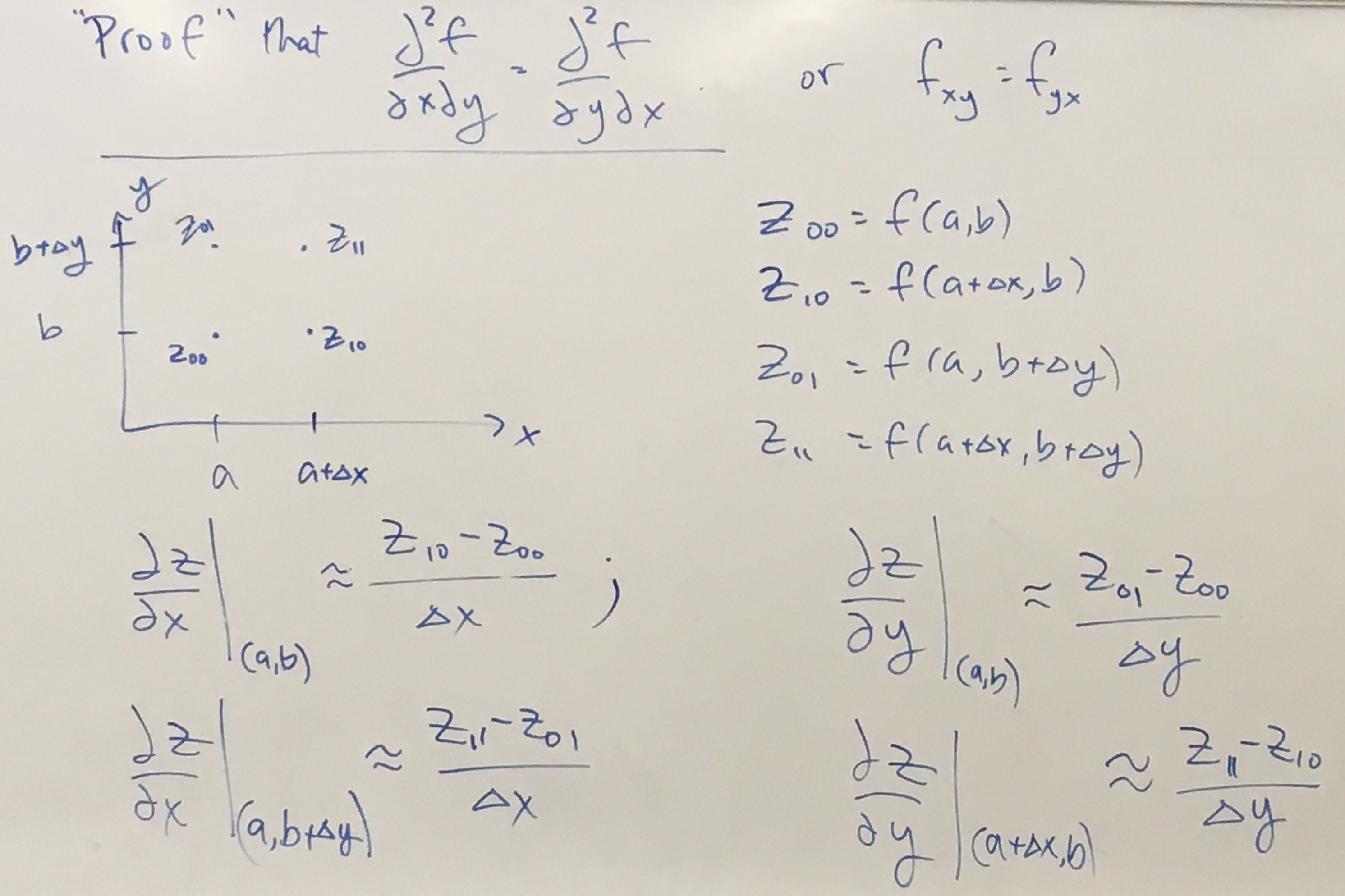
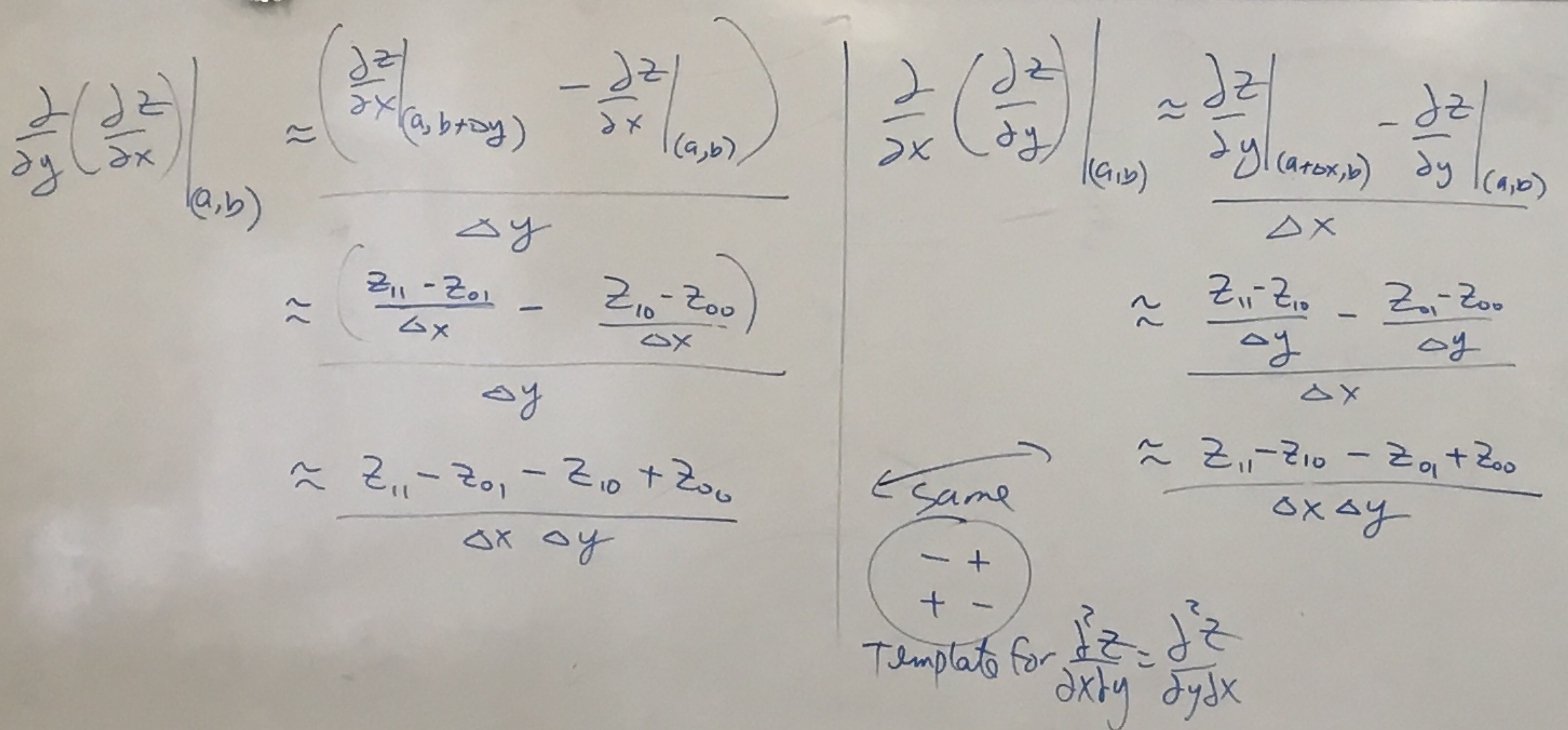
14.3: Partial derivatives
Paul's notes have 3 sections:
Partial derivatives,
their interpretation, and
higher order partial derivatives
Here are pictures of a demonstration that mixed partial derivatives are equal:
page 1 and page 2.
Videos
Partial derivatives
Partial derivative example
Partial derivative from contour plot
Second partial derivatives
Second partial derivatives
Section 14.2: Limits of Real-Valued Functions of Two Variables
Paul's notes
Videos
Limits are...weird..for multi-variable functions
Limits of Functions of Two Variables
Example 1
Example 2
Example 3
Section 14.1: Real-Valued Functions of Several Variables
Paul's Notes.
Here is a reminder about the web-based apps for 3D graphing:
Desmos 3D,
GeoGebra 3D calculator, and (probably the best choice)
CalcPlot3D app.
Feel free to let me know about other apps.
Mathematica is available to you with a site license. Here is a pdf of the level surface in Set 14.1, problem 12, showing the beautiful figures that Mathematica can make. Even though this is a static image, it is much easier to decipher than the figure in webwork.
Here is another view of the level surface from the same problem, using the standard view with \(z\) pointing up. This view is best for choosing from the 6 slices in the WeBWorK problem. This new pdf also shows the slices with \(x, y\) or \(z = 0\) in blue. For example, you can count 2 slices down from the blue \(z = 0\) slice to see the slice at \(z = -1\). (The distance between slices is \(\Delta x, \Delta y\), or \(\Delta z = 0.5\).)
Hint: Consider the symmetry of the surface. For example, the slices at \(x = -1\) and \(x = 1\) look the same. Also, the four slices at \(z = \pm 1\) and \(y = \pm 1\) all look the same!
See this site with a link to
Mathematica at NAU.
You can get Mathematica for your own computer!
Videos
Finding domain
Level curves, contour plot
Function value from contour plot
Increasing or decreasing from contour plot
Traces
Graph Two Variable Function with 3D Calc Plotter
Contour plot with 3D Calc Plotter
Midterm 1 will be in class on Tuesday, Sept. 24.
The solutions to the quiz from Sept 13 are posted on the "files" page at Canvas.
A sample Midterm 1 with solutions will be posted there soon.
Section 13.3 and 13.5: Speed, velocity, and acceleration
Paul's notes
Videos
Velocity, speed, direction, and acceleration
Velocity and Position from Acceleration
Section 13.2: Calculus of vector-valued functions
Paul's notes
Videos
Derivative of vector-valued functions
Properties
More properties
Equation of tangent line
Angle of two curves
Integration with Initial Conditions
Definite integral
Section 13.1: Vector-valued functions
Paul's notes
Here are 3 different web-based 3D graphing programs:
Desmos 3D,
GeoGebra 3D calculator, and
CalcPlot3D app.
Feel free to let me know about other apps.
Mathematica is available to you with a site license.
Here is a Mathematica notebook, helix.nb,
that will plot a parameterized curve in \(\mathbb{R}^3\).
It is harder to use than some other programs, but the pictures are beautiful.
This Mathemtica notebook will Plot 2 Surfaces And 1 Curve.
Videos
Vector valued functions
Domain of a Vector Valued Function
space curves in 3D Calc Plotter
Curve of intersection of two surfaces
Curve of intersection of two surfaces
Vector Valued Function from a Rectangular Equation
Section 12.7: Cylindrical and Spherical Coordinates.
Here are Paul's notes on
polar,
cylindrical, and
spherical coordinates.
BEWARE! Paul lies to you. He writes the formula “\(\theta = \tan^{-1} (\frac y x )\)”,
which is wrong in two ways: It is false half the time,
and it uses the abominable notation “\(\tan^{-1}\)” instead of “\(\arctan\)”.
Remember, the best single formula we can write is
“\(\tan(\theta) = \frac y x\), provided \(x \neq 0\).”
To compute \(\theta\) you need to draw a darn picture!
Here is a figure about how to compute theta in polar or cylindrical
or spherical coordinates using the picture you have drawn.
For those who prefer a formula,
I wrote this algorithm for finding \(\theta\).
Note that \(\arctan(y/x)\) is undefined if \(x = 0\), so those cases are handled first.
I don't intend you humans to follow this algorithm exactly: Just draw the #!#! picture.
Videos
Cylindrical Coordinates
Spherical Coordinates
Cartesian Coordinates to Spherical
Spherical Coordinates to Cartesian
Cartesian Coordinates to Cylindrical
Cylindrical Coordinates to Cartesian
Cylindrical Equations to Rectangular
Rectangular Equations to Cylindrical
Spherical Equations to Rectangular
Rectangular Equation to a Spherical
Spherical Equation to a Rectangular
Section 12.6: Quadratic Surfaces
Paul's notes
Videos
Cylindrical Surfaces
Quadric Surfaces
Ellipsoid
Elliptical Cone
Elliptical Paraboloid
Hyperbolic Paraboloid
Here are some web-based 3D plotters
desmos 3d is the simplest but is also in beta mode.
CalcPlot3D
has more features, but is consequently harder to use.
Here is a video about how to plot
Surfaces in 3D Calc Plotter.
Section 12.5: Planes in space
Paul's notes
Desmos graph for the line 3x + 2y = 7 in the plane, written as the line through (0, 3.5) with normal vector (3, 2).
Videos
Normal equation of plane
Point of Intersection of a Plane and a Line
Point of Intersection of a Plane and a Line
Intersection to two planes
Line through a point and perpendicular to a plane
Plane given with point and parallel plane
Plane given with three points
Plane given with three points
Plane given with point and orthogonal line
Angle between two planes
Distance between point and plane
Distance between parallel planes
Distance between line and point
Section 12.4: The Cross Product.
Paul's notes
Example: calculation of the cross product done in two ways.
This is my problem 6 on the WeBWorK. You only need to do it one way, but it's comforting that they
give the same answer.
Suggested videos on matrices
Multiplying matrices
2x2 determinant
3x3 determinant
Suggested videos on the cross product
Cross product
Cross product
Cross product example
Area of space triangle
Volume of parallelepiped
Section 12.3: The Dot Product.
Paul's notes
Suggested videos.
Dot product
Angle between vectors
Parallel and perpendicular components
In-class group work. The methane molecule \(C H_4\) has 4 Hydrogen atoms at the vertices
of a tetrahedron, with a single carbon atom at the center. Find the bond angle, which
is the angle between the two vectors from the carbon atom to a hydrogen atom.
These desmos3D graphs should help. Methane molecule, 8 Spheres in a Cube,
and Tetrahedron in a Cube
Here are some formulas needed for the webwork. Only some are in Paul's Notes.
It is easiest to make sense of these formulas using the notation \(\hat{\bf a}\) (pronounced a-hat) for the unit vector in the direction of \(\bf a\). To compute that unit vector, use the formula \(\hat{\bf a} = \frac{\bf a}{\|\bf{a}\|}\).
The component of \(\bf b\) along \(\bf a\) is \(\hat{\bf a} \cdot {\bf b} = \frac{\bf a \cdot {\bf b}}{\| {\bf a} \|}\), which is a scalar.
The projection of \(\bf b\) parallel to \(\bf a\) is \({\bf b}_{\| {\bf a}} = (\hat{\bf a} \cdot {\bf b}) \hat {\bf a} = \frac{({\bf a} \cdot {\bf b}) {\bf a}}{\| {\bf a} \|^2}\), which is a vector. Note that the final expression has no square roots.
The projection of \(\bf b\) perpendicular to \(\bf a\) is \({\bf b}_{\perp {\bf a}} = {\bf b} - {\bf b}_{\| {\bf a}} \), which is a vector.
Note that \({\bf b} = {\bf b}_{\| {\bf a}} + {\bf b}_{\perp {\bf a}} \) must hold (by definition), and it turns out that
\({\bf b}_{\| {\bf a}} \cdot {\bf b}_{\perp {\bf a}} = 0\), so these two projections are orthogonal to each other.
Section 12.2: Vectors in \(\mathbb{R}^3\)
Paul's notes
Suggested videos.
Parametric equation of line in 3D
Parametric equation of line in 3D
Intersection of two lines
Section 12.1: Vectors (Note: The section number 12.1 follows the Rogowski and Adams textbook.)
Paul's notes on
basics and
vector arithmetic.
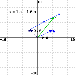
The answer to one version of WeBWorK problem 10 in set 12.1 is
x = a + 1.6 b. (So type 1 and 1.6 into the two blanks.)
This figure shows the vectors.
Here is a Mathemetica notebook to allow arbitrary linear combinations of
a and b.
Suggested videos.
Vector operations: Sum, scalar multiple, dot product
Length of a 3D vector
Unit vectors: Direction of a vector
Plotting points