MAT 667, Dynamical Systems

Contact information

My office phone, 523-6878, goes straight to voice mail.  You can send me e-mail at Jim.Swift@nau.edu. Here is my weekly schedule.
Please feel free to contact me any time via e-mail with any questions about the math, or with any feedback about the class.

Office hours are usually in my office, AMB 110. Occasionally I will be down the hall in the MAP room (AMB 137). If I am not at my office during office hours, look for me there.
Tu: 11:30-12:30
W: 11:30-1:00
Th: 2:45-3:45
F: 11:30-1:00
You can always send me e-mail, drop in to my office, or make an appointment if these times aren't convenient.

Darryl Nester's Slope Field Applet.

Chart of letters of the Greek alphabet.

Associated materials in reverse chronological order

Monday, May 1
Lyapunov Exponents and Lyapunov numbers.
Page on the graph of Lyapunov Exponents for the Logistic Family of Maps.
For Lyapunov numbers for 2-dimensional maps we need to understand the image of a ball under a linear transformation. It is an ellipse, as shown in this A times Ball Mathematica notebook.

Wednesday and Friday, April 26 and 26 Presentations

Monday, April 24
A formula for \(Df^k(x_0)\) for \(f: \mathbb R^n \to \mathbb R^n\). Stability of the period 2 orbit in the standard map.
Here is the animated gif of that periodic orbit, from March 8.
Use the Standard Map app to look at the standard map with \(k = 2.1\). We have found that the period 1 point has eigenvalues \(\pm i\) and the period 2 points have eigenvalues \(-1, -1\) when \(k = 2\).

More about the Bifurcation Diagram for the Logistic map.
Using Mathematica to find the period 4 and 8 branches of the Logistic map, and the Feigenbaum constants.

Friday, April 21
Start looking at the bifurcation diagram for the Logistic Map, starting with period one and 2 points. The Mathematica notebook Period1and2stability.nb shows the result of what was done in class.

Wednesday, April 19
A formula for \((f^k)'(x_0)\) for \(f: \mathbb R \to \mathbb R\). Here's a scan of the whiteboard.

Monday, April 17
Stability of the Origin in the Standard Map. Here is the javascript app of the Standard Map.

Wednesday, April 12, Friday April 14
Sinks, stability of fixed points and periodic orbits in terms of derivatives.
Updated Iterated Maps pdf.

Monday, April 10
More about iterated maps, including circle maps, and their rotation number. Here is my mathematica notebook circleMap.nb.

Friday, April 7
More about iterated maps. Here is pdf about Iterated Maps based on my lectures. The definition of a sink is motivated by these examples: notSink.nb.

Wednesday, April 5
More detail about one-dimensional maps. Read Simple mathematical models with very complicated dynamics, by Robert May. This article was influential in the 1970s. A few notes about this article. The images in Figures 2 and 3 are switched, although the captions are correct. Also, May mis-understood an important result: For the Logistic map, IF there is a stable periodic orbit, then \(x = 0.5\) is in its basin of attraction. May states a few times that there an attracting periodic orbit for any value of \(a\).

Monday, April 3
Ideas for projects.
Here is a link to an electronic copy of a textbook I have used for this class in the past: Chaos: An Introduction to Dynamical Systems, an e-book, supplied by Cline Library. It has some ideas for projects.

Friday, March 31
The Poincare Map for the shaken washboard (the driven damped pendulum).
ShakenWashboard2.nb Mathematica Notebook. This shows the Poincare map on a program similar to ShakenWashboard1.
ShakenWashboard3.nb Mathematica Notebook. This has only the Poincare map, and allows a larger number of iterations.

Monday, Wednesday, March 27, 29 The Shaken Washboard, both the Actual Shaken Washboard (ASW) and the ODE model.
ShakenWashboard1.nb Mathematica Notebook.

Wednesday, Friday, March 22, 24 More about the standard map and the Shaken Washboard
Here's a recording of part of Friday's class, showing how to make an animated gif of the kicked rotator (standard map) using the mathematica notebook standardMap.nb

Monday, March 20
Homework 2
Here's a youtube video of a Driven Damped Pendulum Analog, also known as the shaken washboard.
These videos allow us to estimate the friction constant of the green marble and the yellow ball.

Wednesday, Friday, and Monday, March 8, 10, 20
The standard map. Here is a web site with an interactive app which uses javascript.
Here are some animations made with my standardMap.nb Mathematica notebook.
k = anything, period 2,   k = pi/2, period 6. This was on the whiteboard giving the \((\theta_n, \omega_n)\) coordinates of that period 6 orbit with \(T = 5\) and \( \Delta \omega = \pi/10\).
k = 0.7, period 10,   k = 0.05, period 60, k = 0.05, period 40. (These last two have a kick every frame. \(T = 0.1\))
These last animations are reminiscent of the way Isaac Newton modeled gravity by a sequence of impulses. That image is from this book

Monday, March 6 More about driven, damped linear oscillators.
Computation of the periodic particular solution using complex variables

Friday, March 3 More about driven, damped linear oscillators.

Wednesday, March 3 Snow Day!

Monday, February 27 More about driven, damped linear oscillators.
NIST web page about the Quality Factor,Q
Desmos animation of a Shaken Mass on a Spring.
Desmos graph of the Resonance Curve, showing Full Width at Half Maximum Power.

Friday, February 24
Review of ODEs (MAT 239), with a focus on the driven, damped, linear oscillator.
Here is the relevant part of my web page from MAT 239.
I will also use complex variable techniques to make all of the calculations simpler.

Wednesday, February 22 Snow day!

Monday, February 20
Scaling for Newton's Law of Cooling for an object in an oscillating ambient temperature. Here is a graph of solutions to the dimensionless equations, with a caption.

Friday, February 17
Scaling of ODEs and maps.
Example from Newton's Law of Cooling. After class, I did this calculation get a dimensionless verion Newton's Law of Cooling, with no parameters.
Homework 1 The latest is version 3, with changes in red. Version 2 has an equation corrected to \(t = \beta \bar t\) in problem 1(c).

Wednesday, February 15
More about Area Preserving Maps.
The Poincare map for a Conservative (Hamiltonian) system of ODEs, like the double pendulum, is an area preserving map.

Monday, February 13
Overview of Area Preserving maps, with a focus on the Standard Map.
Video of Jim Meiss talking about the Standard Map. Here is a page with his computer program that only works for Mac OS 10.14 or earlier. (My laptop has Mac OS 12.6.2.) That link also has some useful mathematical information, though.

Wednesday, February 8, 10
Overview of complex dynamics: the Newton fractal, the Mandelbrot set, and "The Splendor and Science of Chaos"

Monday, February 6
Overview of Circle maps

Monday, January 30 and February 1, 3
Overview of the Logistic map.
Takashi Kanamaru's Logistic Map Time Series. This shows the cobweb diagram and the time series. You *might* be able to run the Java program after saving it to disk.
Here is a Bifurcation Diagram from the wikipedia page on the logistic map.
Here is my bifurcation diagram and skeleton as printed on the LMC wall. The bottom shows the first few iterates of x0 = 0.5. Unfortunately, the detail in the upper right corner was not printed. A small version of the proper diagram is posted in the AMB near the mail room.
This page of the Logistic Map has another version of the bifurcation diagram for the LMC wall.
Mark Haferkamp's cobweb diagram generator. This was a project when Mark took MAT 667 in 2017.
Takashi Kanamaru's Logistic Map Bifurcation Diagram. You can zoom in to observe Feigenbaum's universal constants, \(\delta \approx 4.669\) and \(\alpha \approx -2.503\).
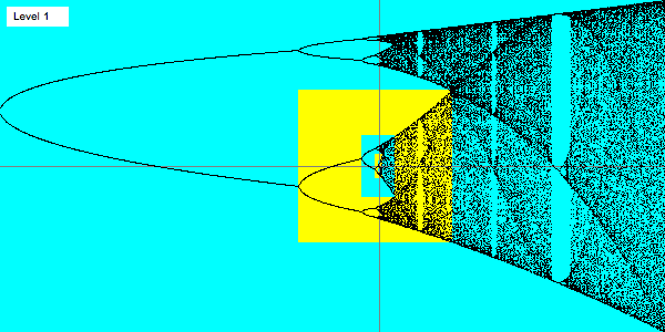
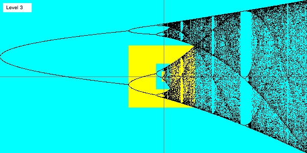
These are similar I made:
Here is an animation with 3 bifurcation diagrams with \( 3 \leq a \leq 4\) (level 1), then level 3 (period doubing 4 to 8 at left, 4 to 2 band merging at right) and level 5 (period doubing 16 to 32 at left, 16 to 8 band merging at right)
Here is an animation with 2 bifurcation diagrams (levels 3 and 5).
Here is an animation with 200 frames (zooming from level 3 to level 5).
My Mathematica notebook, iteratedMap1D.nb

Monday, January 23 (Day 2, 3)
Here is a link to the 1963 paper by Lorenz.
My page on the Lorenz attractor.
Mark McClure visualization Shows convection cells and has the round button (rounds \(\pi\) to 3.142, etc.)
Hendrik Wernecke Simulation. Simple app with only STOP, Reset, and a slider for \(\rho\). This uses Euler's method.
Malin Christersson simulation. Swarms of butterflies!

Friday, January 20 (Day 1, 2)
Double Pendulum Simulation by Eric Neumann