syllabus. Here is a link to NAU policy statements. These math department policies are part of the syllabus for our course.
Link to text, Chaos: An Introduction to Dynamical Systems, an electronic resource of the entire book, supplied by Cline Library. (You need to be logged in from an NAU domain, possibly VPN.)
Office hours: MTWF 10:30-11:20.
Marek Rychlik's Slope Field Applet, at Eduardo Sontag's web site.
My links to external Chaos Sites.
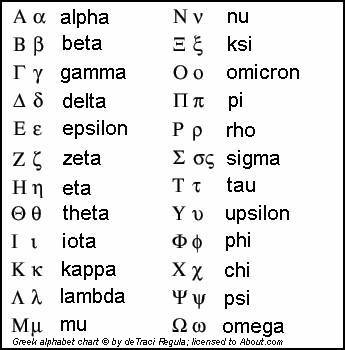
Chart of letters of the Greek alphabet.
May 9
Mark Haferkamp's cobweb diagram generator.
(This doesn't work in Internet Explorer.)
May 3:
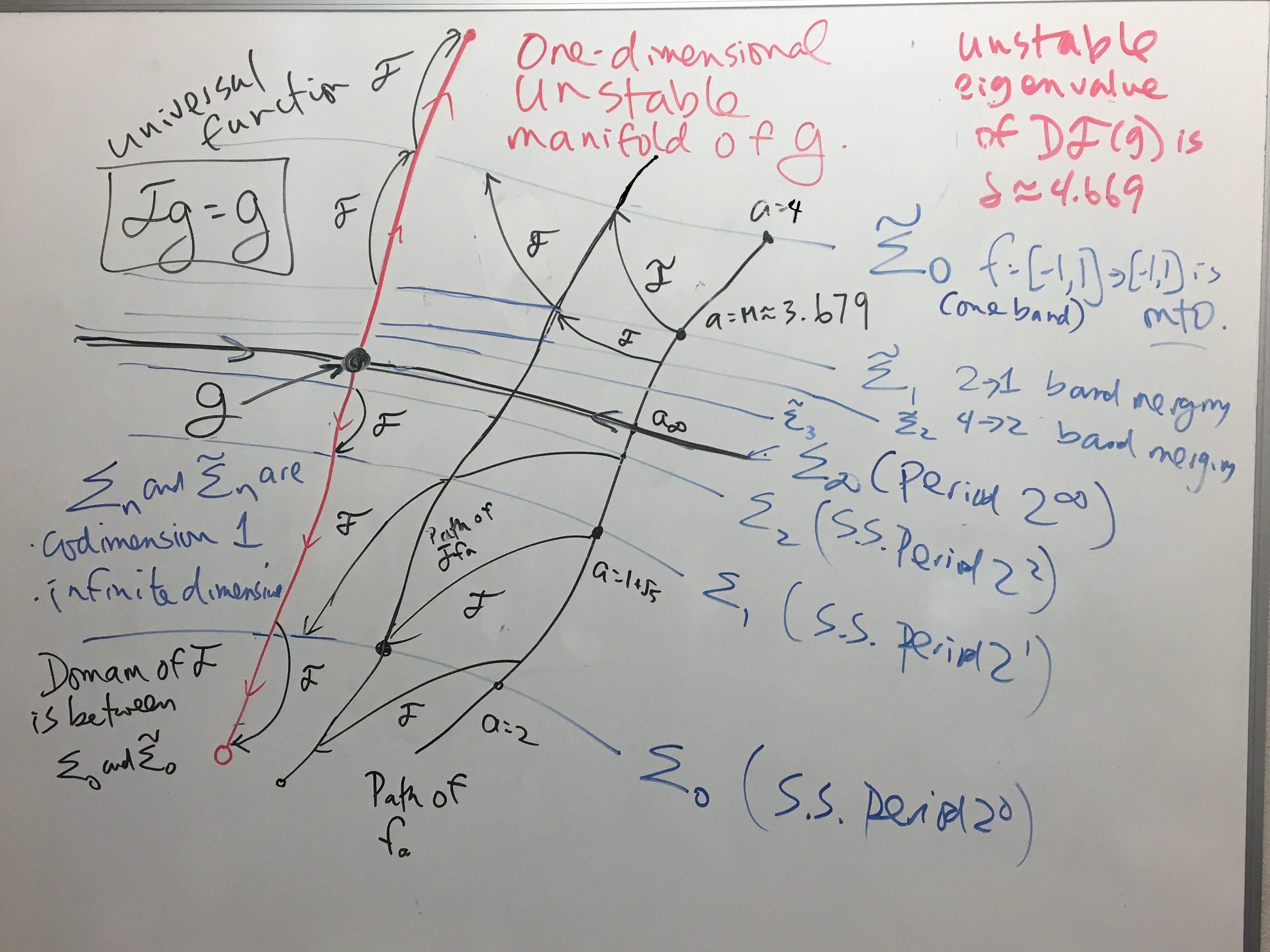
The Period Doubling Operator. This is my notation, which is not common. Most people define the domain of T to be a subset of all functions with f(0) = 1.
My domain has f(-1) = f(1) = -1.
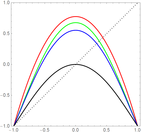
Figure of logistic map f_a with superstable period 8 (red), Tf (green), T^2 f (blue) and T^3 f (black).
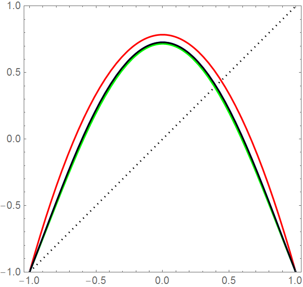
Figure of logistic map f_a at accumulation of period doubling (red), Tf (green), T^2 f (blue, hidden) and T^3 f (black).
The figure explaining Feigenbaum's universality.
April 26:
HenonMapEigenvaluesPer2too.nb showing period doubling bifurcation of the period 2 orbit.
(For Problem 2.7 in HW 4.)
Homework 6 due Wednesday, May 3.
hw 6 Help.nb Mathematica notebook to help with Homework 6.
Doubling Operator 1.nb Notebook about the Feigenbaum/Lanford Doubling operator.
April 19:
period3itineraries.nb
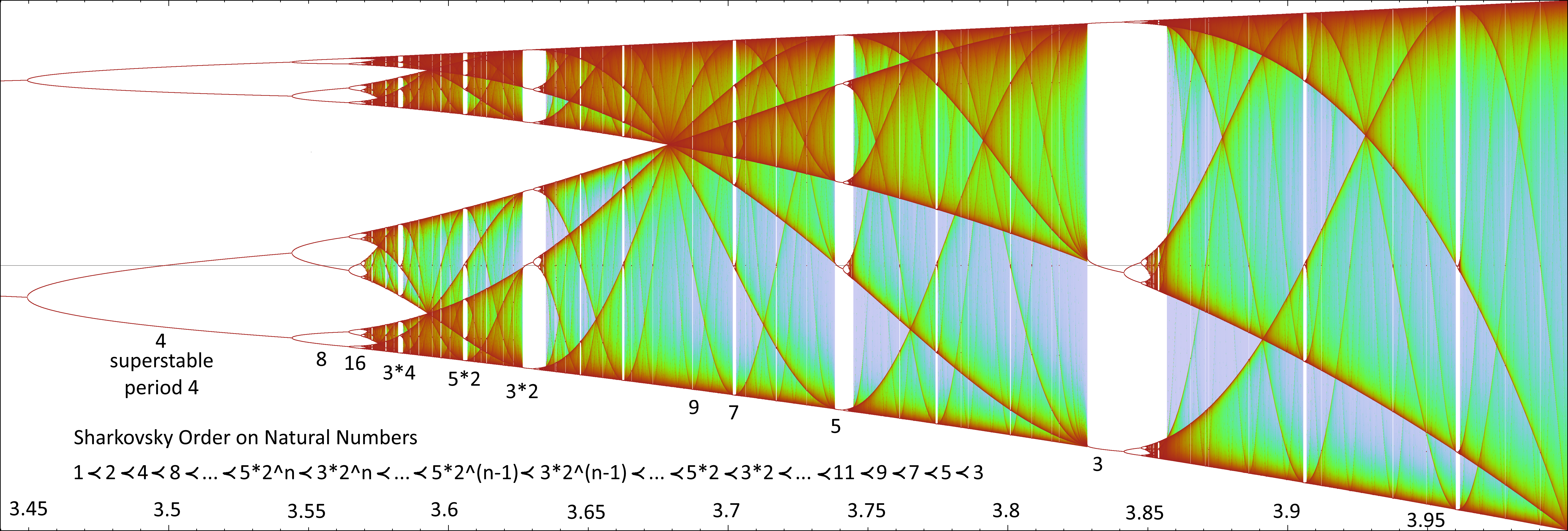
My image showing the Sharkovsky order (1964) in the family of logistic maps.
Here is a Scholarpedia article about the Sharkovsky ordering.
Table from Metropolis, Stein and Stein (1974) showing all superstable orbits with period ≤ 6. In the table, L = [0, 1/2) and R = (1/2, 1],
and RL2 means there's a superstable period 4 orbit with x1 = 1/2, x2 ∈ R, x3 ∈ L, x4 ∈ L
(and x5 x1= 1/2 for superstable period 4).
April 10:
Homework 5 due April 19.
April 7:
Page on the graph of Lyapunov Exponents for the Logistic Family of Maps.
April 5:
A handout on the web with nice graph of the Lyapunov exponent as a function of the parameter, for the Logistic map.
(By Peter Young at UCSC.)
April 3:
logisticMapConjugacy.nb Mathematica notebook.
March 29:
Attractors of the Whitley Map.
March 27:
Mathematica notebook WhitleyMapEigenvalues.nb.
March 24:
A times Ball Mathematica notebook. The image of a ball under a linear transformation is an ellipse (or ellipsoid, possibly degenerate).
March 22:
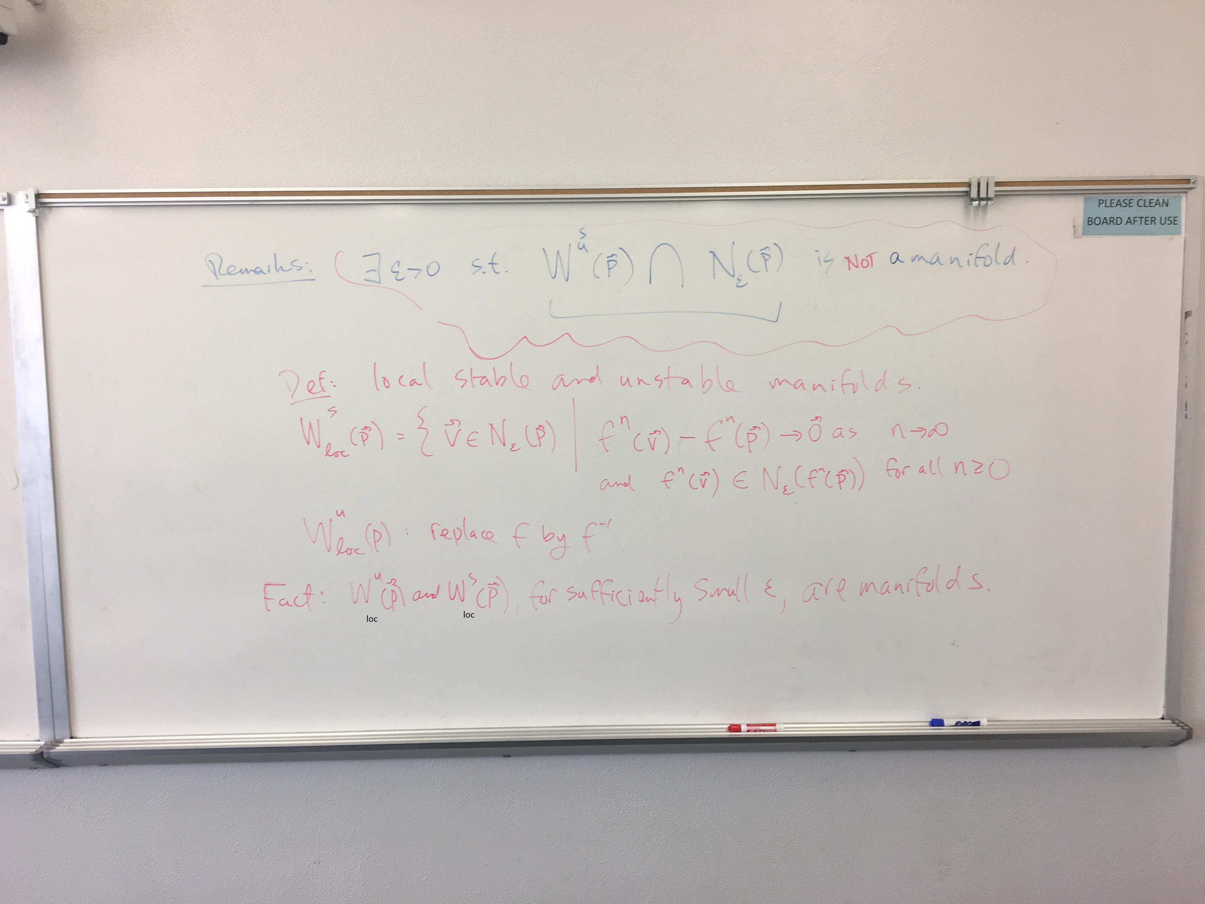
Correction to lecture about stable manifolds and local stable manifolds.
March 20:
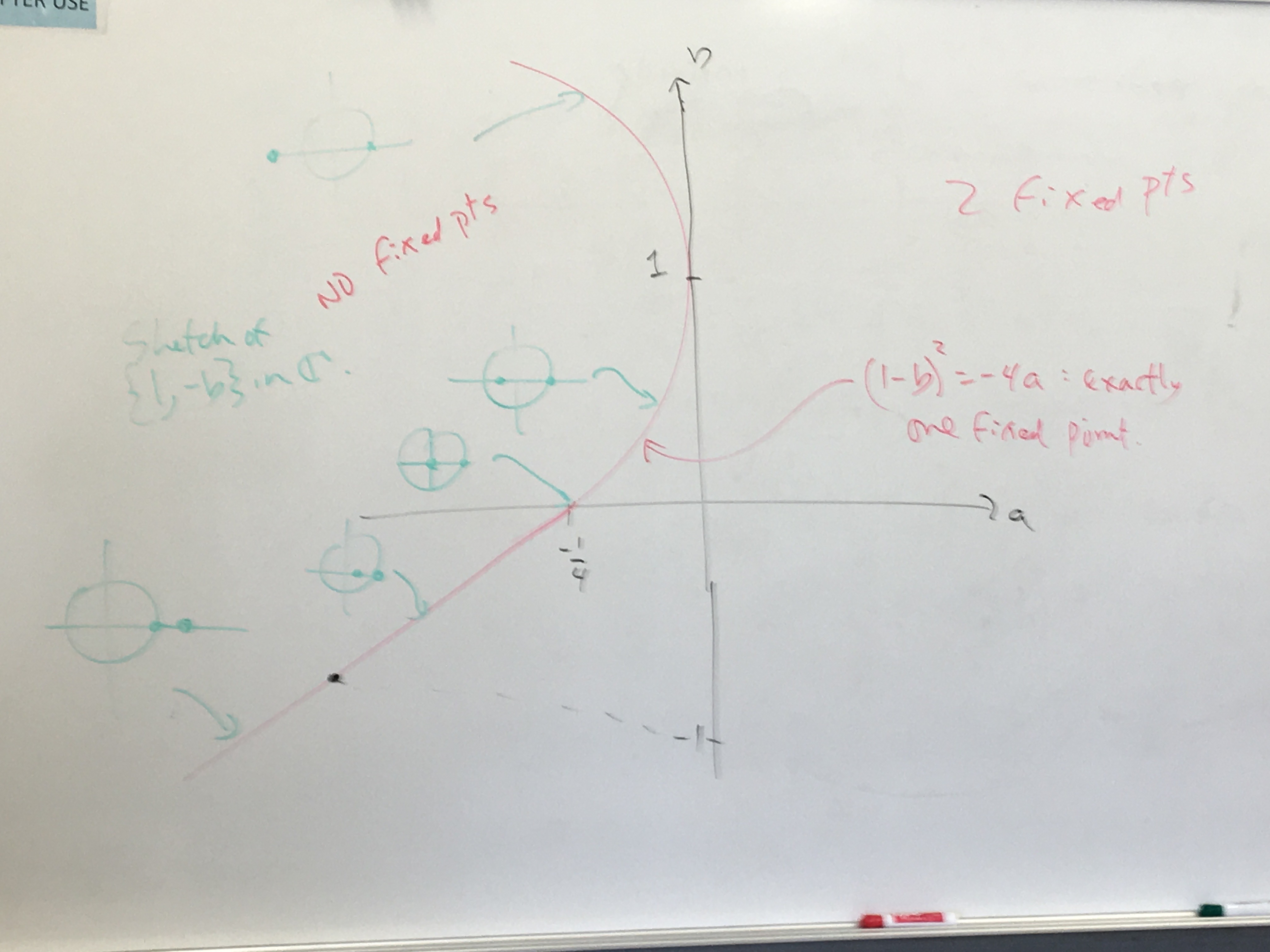
Photo of the Henon Parameter Plane on the whiteboard Friday before break.
Mathematica notebook HenonMapEigenvalues.nb.
March 10:
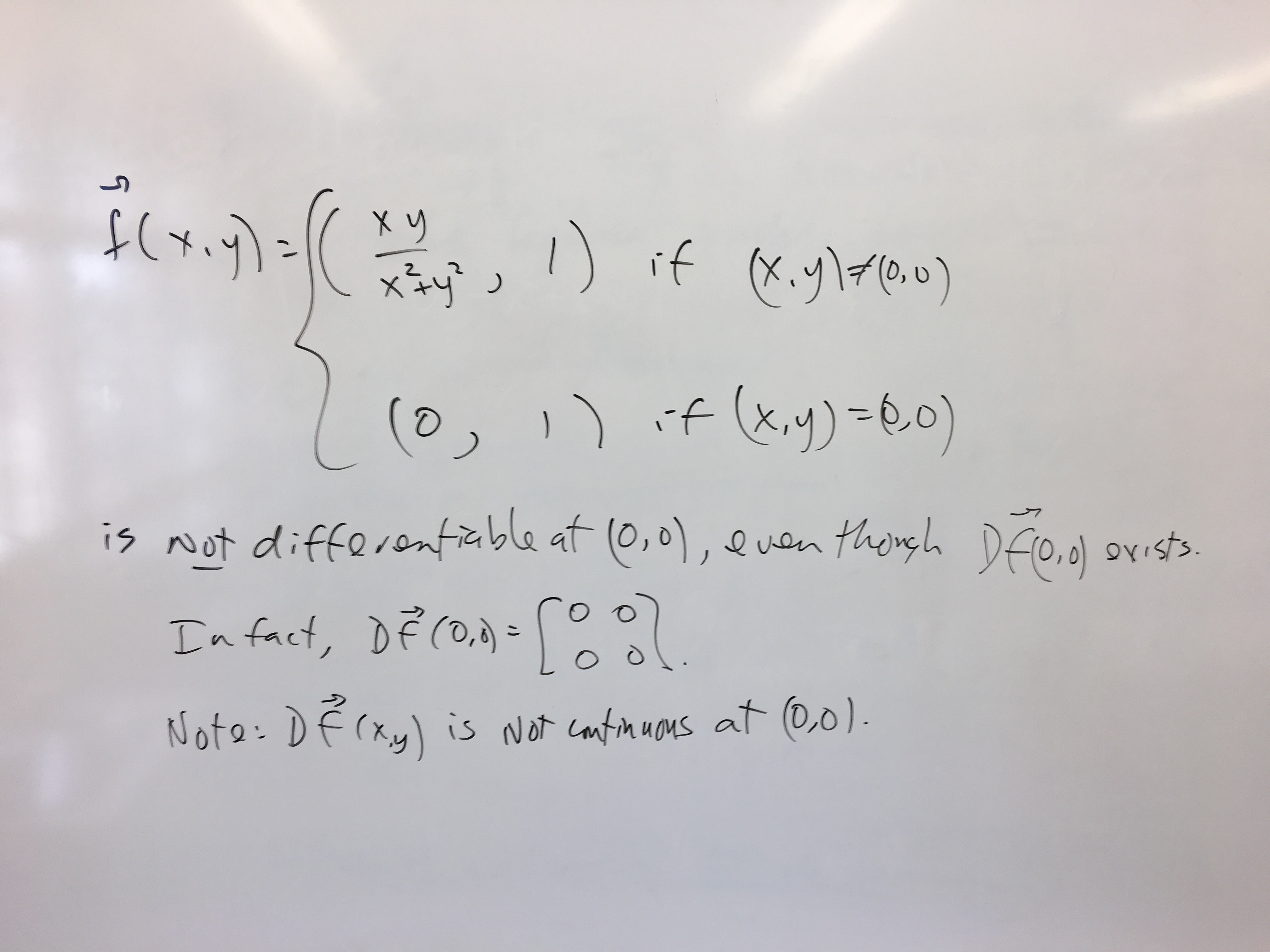
After class I found an
example of a function mapping R2 to R2 that is not differentiable at (0,0), but all 4 partial derivatives exist at (0,0),
so the Jacobian matrix is defined at (0,0).
March 6:
Homework 4, due Monday March 27.
(hw4.pdf was updated 3-06 at 1:08 pm with F_0 = 0.)
February 24:
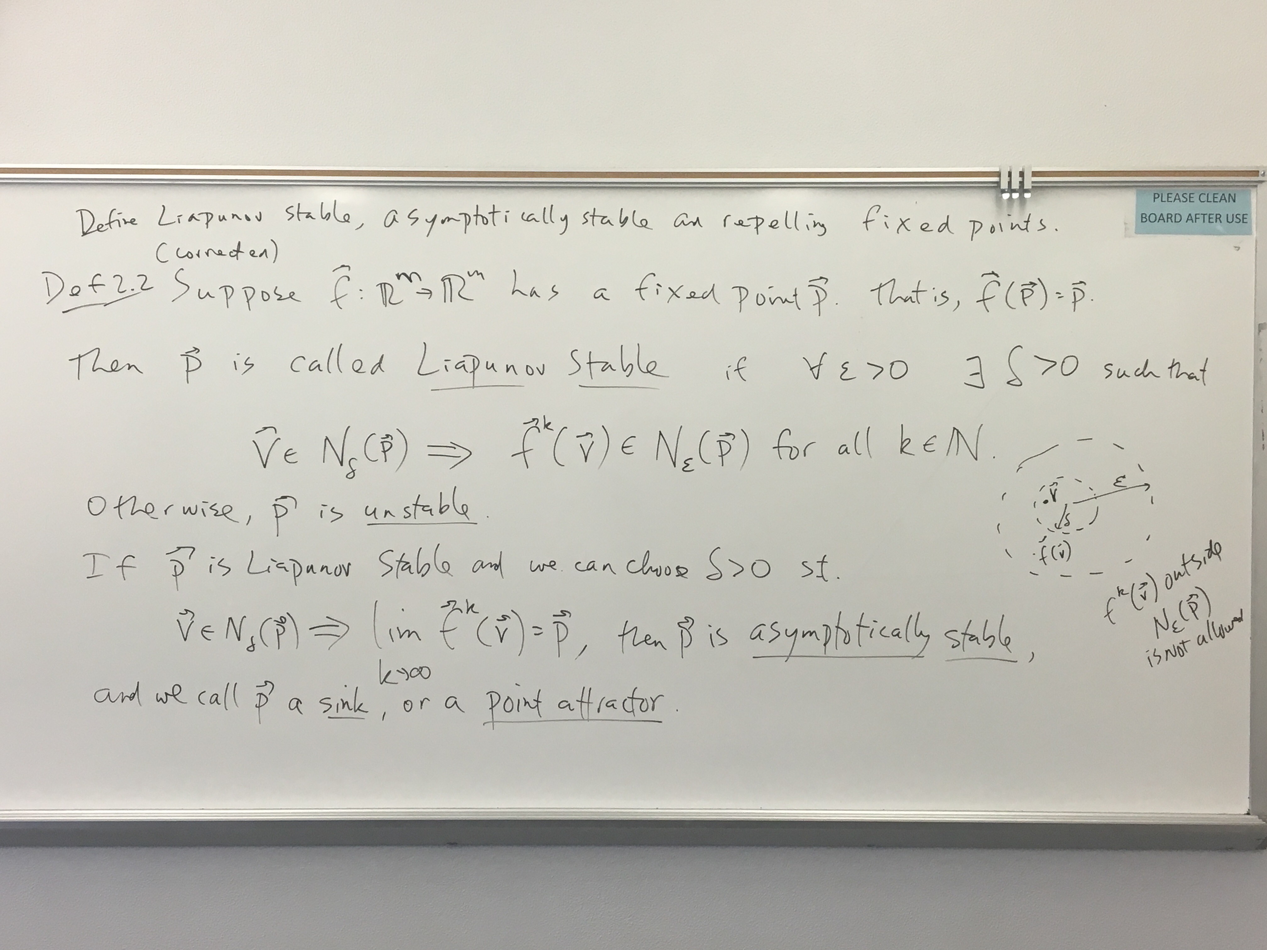
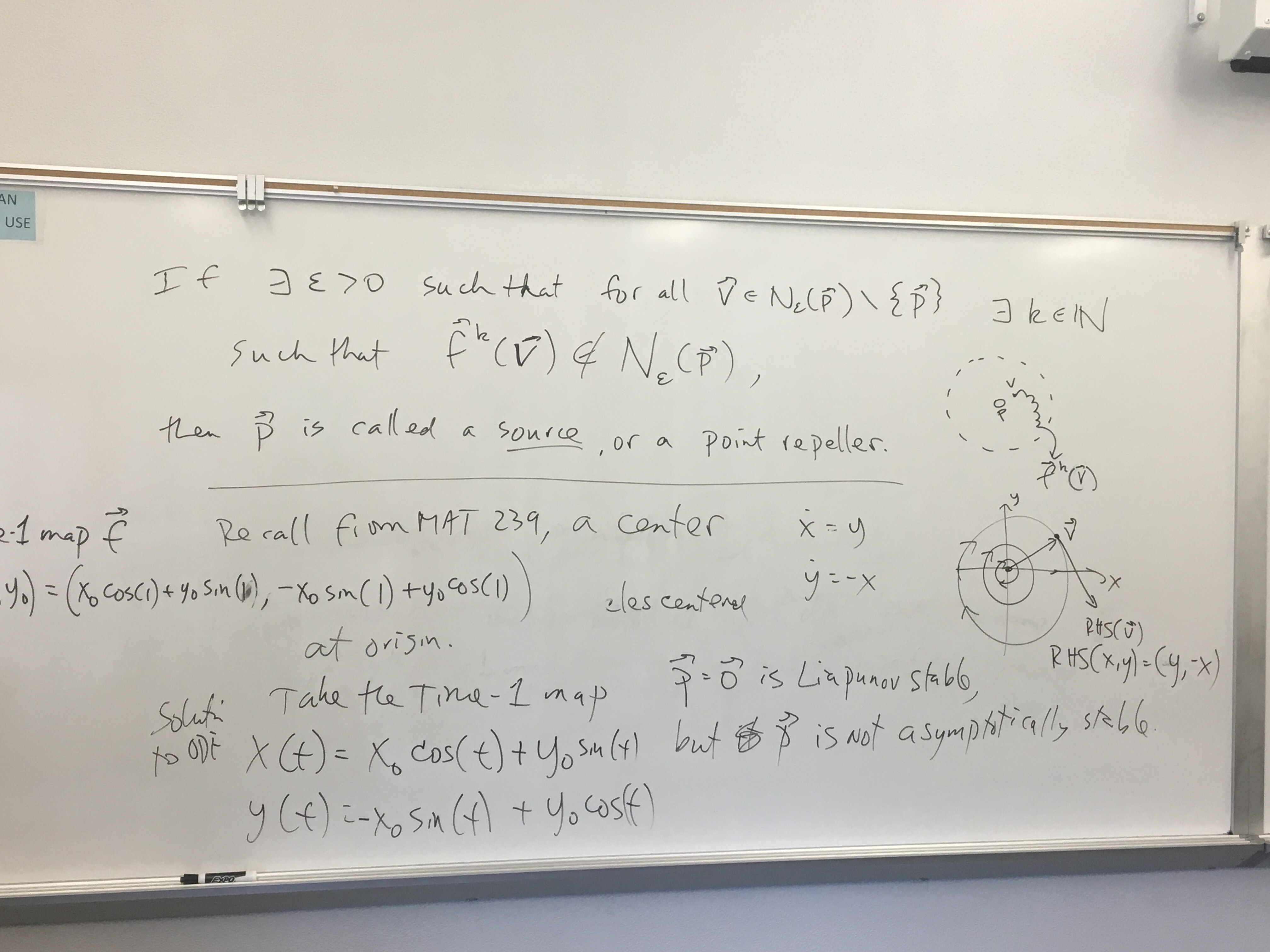
Since I am using a slightly different version of Definition 2.2 from the book, I've taken pictures of the white board so we have the definitions recorded:
Part 1 and Part 2.
February 22:
A previous classes contributions for attractors of the Whitley Map.
February 20:
Mathematica notebook iterated2Dmap.nb.
February 15:
Large bifurcation diagram for the Logistic map.
February 13:
A proposal for the first presentation is due Monday, Feb. 20. (Can be handwritten, email, even a beamer or powerpoint file.)
Mathematica notebook sensitiveDependence.nb to accompany the proof sensitive dependence in the doubling map.
February 10:
Homework 3, due Monday, February 20.
February 8:
17 Equations that changed the world
Homework 3 to appear soon!
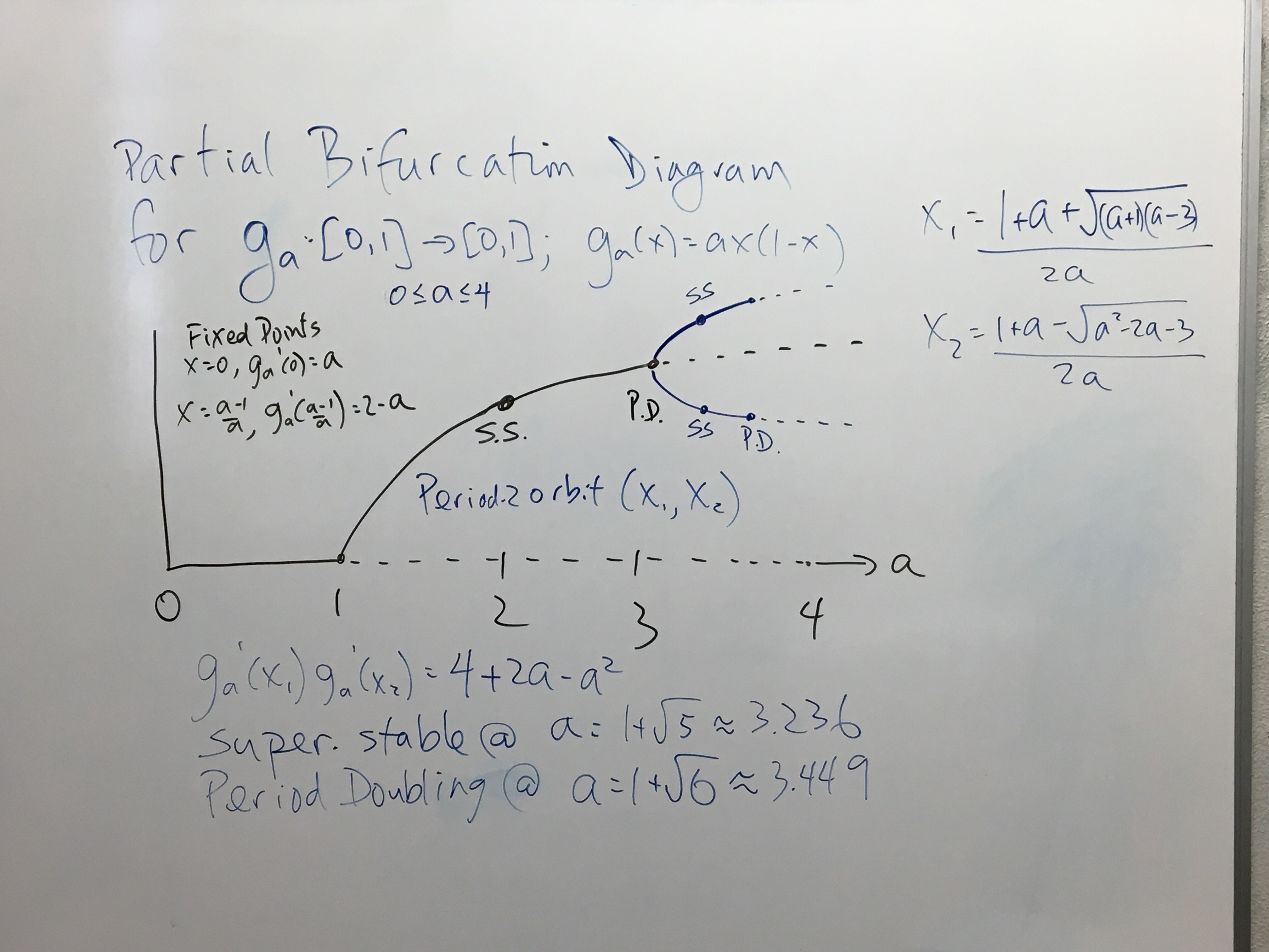
Partial Bifurcation Diagram of the Logistic Map.
January 27:
Homework 2, due Monday, February 6.
Mathematica Notebook interatedMap1.nb
January 20:
Homework 1, due Wednesday, January 25.
Mathematica notebook DrivenDampedPendulumClassContributions.nb. (Open DrivenDampedPendulum.nb from Jan 18 first.)
Mathematica notebook DrivenDampedPendulum2.nb.
c = 0.5, rho = 1.4917: Jeffrey's contribution.
c = 50, rho = 5: Shehara's contribution.
c = 1/3, rho = 2: Jimie's contribution.
c = 0.5, rho = 1.69: Scott's contribution.
c = 0.5, rho = 0.9: Philip's contribution.
c = 0.5, rho = 10: AllisonL's contribution.
c = 1, rho = 2.04: Jim's contribution.
c = 1, rho = 1: Jim's contribution of an unstable periodic solution.
January 18:
Takashi Kanamaru's Logistic Map Applet, and
Logistic Map Bifurcation Diagram.
The following animated gifs were all made by the Mathematica notebook DrivenDampedPendulum.nb.
They all have the parameters w = 2Pi and w0 = 1.5*2Pi. The other parameters are:
c = 0, rho = 0: undriven, undamped, small amplitude (Use the back button to get back.)
c = 0, rho = 0: undriven, undamped, large amplitude
c = 0, rho = 0: undriven, undamped, rolling motion
c = 0.1, rho = 0: undriven, damped
c = 0.5, rho = 1.06: driven, damped, period 1 transient
c = 0.5, rho = 1.06: asymmetric period 1
c = 0.5, rho = 1.073: period 2
c = 0.5, rho = 1.077: period 3
c = 0.5, rho = 1.4: rolling motion
c = 0.5, rho = 1.503: chaos
Homework Due Thursday, Jan. 19 at 11:59pm. Send me an animated gif made by this program, showing something you find interesting.
Give me the parameters you used, for example copy and paste the cell you used
into the email. Indicate if I can post to the website using your name, or not.