The official textbook,
Whitman,
is freely available online.
Another free textbook
Herman and Strang,
is on OpenStax.
If you want to get a physical textbook, we recommend any edition
of Calculus, Early Transcendentals, by Rogawski et al.
There many freely available resources on the internet, for example the
Paul's Notes,
by Paul Dawkins of Lamar University,
and wonderful videos at the Khan Academy
There are videos and other resources at the MOOCulus site,
https://mooculus.osu.edu/.
Here is a link to NAU policy statements, and the math department policies that are technically part of the syllabus.
An excellent web-based calculator is www.desmos.com/calculator
Most homework is assigned and graded using WeBWorK. Your username and password is the same as for LOUIE. (A typical username is abc123.) Use any WeBWorK link at this web site, or type in https://webwork.math.nau.edu/webwork2/JSwift_136/.
This link has detailed information on WeBWorK (in pdf format). Your username and password are the same as for Louie.
Chart of letters of the Greek alphabet.
I hope you will come to my office hours to introduce yourself. Aside from my office hours, we have lots of free help available.
The Math Achievenment Program (MAP) room is just 20 or 30 yards north of our classroom, in AMB 137.
Starting September 6, it will be open M-Th 10-6 and F 10-2. This is staffed by Peer Math Assistants (PMAs), and I will also have some of my office hours there.
Free drop in tutoring and one-to-one tutoring is available at the North and South Academic Success Centers.
Monday, December 5: Set 25, Substitution
In-class worksheet on
the method of \(u\)-substitution, with the
scanned solutions.
Wednesday, November 30: More about Set 25, Net Change as an Integral
Here is a picture of the whiteboard showing formulas about Total Change (also called net change) and
displacement and distance traveled.
Monday, November 28: Set 25, Net Change as an Integral
This set is about applications of the FTC.
The worksheet today is from the sample Midterm 4, which was handed out in class.
Wednesday, November 23: More on set 24, The Fundamental Theorem of Calculus, Part 2
Here is the Big Picture of Calculus.
In-class worksheet on solving the initial value problem
\(\frac{dy}{dx} = f(x), y(x_0) = y_0\), with the
scanned solutions.
Here is a
Slope Field Applet
for solving initial value problems graphically.
Monday, November 21: Set 24, The Fundamental Theorem of Calculus, Part 2
In-class worksheet on
The Fundamental Theorem of Calculus, Part II, with the
scanned solutions.
Friday, November 18: More on set 23, The Fundamental Theorem of Calculus, Part 1
Proof of the Fundamental Theorem of Calculus, Part I.
In-class
Quiz 8, with the
scanned solutions.
Thursday, November 17: Set 23, The Fundamental Theorem of Calculus, Part 1
In-class worksheet on
The Fundamental Theorem of Calculus, with the
scanned solutions.
Wednesday, November 16: Set 22, The Indefinite Integral
In-class worksheet on
The Indefinite Integral, Part 2, with the
scanned solutions.
Monday, November 14: Set 22, The Indefinite Integral
In-class worksheet on
The Indefinite Integral, with the
scanned solutions.
Thursday, November 10: Set 21, Area and the Definite Integral
The definition of the Definite Integral, and some of its properties.
For the Limit Definition of the Definite integral see
Paul's Notes.
I also have a
scan of the whiteboard
from Thursday, but it is barely readable.
Sorry! I scratched the lens on my phone.
Wednesday, November 9: Set 21, Area and the Definite Integral
In-class worksheet on
The Definite Integral, with the
scanned solutions.
Thursday, November 3: Set 20, Optimization and Newton's Method
Here is a YouTube video of me showing how to do
Mewton's Method with a Spreadsheet.
Wednesday, November 2: Set 20, Optimization
The key is setting up a function of one variable, \(Q = f(x)\),
whose output \(Q\) is the thing you want to optimize. Here are some steps:
(1) Understand the problem (Read it carefully, and frequently)
(2) Draw a diagram. Identify the given fixed quantities, and the variable quantities.
(3) Introduce notation. The word "Let" is super-important.
(4) Write the quantity you want to optimize (we will call it \(Q\)) in terms of other quantites.
(5) Usually \(Q\) will depend on more than one quantity.
Use the constraints to eliminate all but one variable quantity to get \(Q = f(x)\).
Write down the domain of \(f\).
(6) Use calculus to find the global max (or min) value of \(f\),
or the input \(c\) at which the global extremum occurs. Read the question again
and answer it.
Monday, October 31: More on set 19, L'Hospital's Rule
The indeterminate forms are
\( \frac 00,~ \frac{\infty}{\infty},~ 0\cdot\infty,~ \infty - \infty,~ 0^0,~ 1^\infty, \text{ and } \infty^0 .\)
L'Hospital's rule can only be used for limits of type \(\frac 00\) and of type \(\frac{\infty}{\infty}\).
In-class worksheet on
Indeterminate Forms, with the
scanned solutions.
Friday, October 28: Set 19, L'Hospital's Rule
L'Hospital's Rule, also written L'Hôpital's Rule, says that if \(\displaystyle \lim_{x \to a} f(x) = \lim_{x \to a} g(x) = 0\), or \(\displaystyle \lim_{x \to a} f(x) = \pm \infty\) and \(\displaystyle \lim_{x \to a} g(x) = \pm \infty\), then
\(\displaystyle \lim_{x \to a} \frac{f(x)}{g(x)} = \lim_{x \to a} \frac{f'(x)}{g'(x)}\)
See the details at
L'Hospital's rule.
In-class
Quiz 7, with the
scanned solutions.
Wednesday and Thursday, October 26 and 27: Set 18, The Shape of Graphs
Definition: A function \(f\) is concave up on an interval \(I\)
provided that \(f'\) is increasing on \(I\).
A similar definition holds for concave down.
Let \(I\) be an interval in what follows.
If \(f' > 0\) on \(I\), then \(f\) is increasing on \(I\).
If \(f' = 0\) on \(I\), then \(f\) is constant on \(I\).
If \(f' < 0\) on \(I\), then \(f\) is decreasing on \(I\).
If \(f'' > 0\) on \(I\), then \(f'\) is increasing on \(I\), and \(f\) is concave up on \(I\).
If \(f'' = 0\) on \(I\), then \(f'\) is constant on \(I\), and \(f\) is straight on \(I\).
If \(f'' < 0\) on \(I\), then \(f'\) is decreasing on \(I\), and \(f\) is concave down on \(I\).
Definition: A turning point of \(f\) is a point on the graph, \((c, f(c))\), provided that \(f\) has a local extremum at \(c\).
Definition: An inflection point of \(f\) is a point on the graph, \((c, f(c))\), where the concavity of \(f\) changes.
Theorem: If \(f''(c) = 0\), and \(f''\) changes sign at \(c\), then \((c, f(c))\)
is an inflection point of \(f\).
This is an application of the First Derivative Test to \(f'\).
Note that if \(f''(c) = 0\), then
\( (c, f(c)) \) is not necessarily an inflection point of \(f\).
Consider those functions \(f\) with \(f''(x) = x^2\), which have \(f'\) increasing, and \(f\) concave up, on \( (-\infty, \infty)\).
In-class worksheet on the Shape of Graphs, with the scanned solutions. Here is a desmos graph of \(y = e^{-x^2/2}\)
Monday, October 24: Set 17, Critical Points and Local Extrema, and the Mean Value Theorem.
Definition: A function \(f\) is increasing on an interval \(I\)
provided that \(f(x_1) < f(x_2)\) for all \(x_1 < x_2\) in \(I\).
A similar definition holds for decreasing.
Theorem: If \(f'(x) \geq 0\) for all \(x\) in an interval \(I\),
and \(f'(x) = 0\) only at a finite number of points (possibly no points),
then \(f\) is increasing on \(I\).
A similar theorem holds for \(f(x) \leq 0\) and \(f\) decreasing.
Examples: We can see from the definition that \(f(x) = x^2\) is increasing on \( [0, \infty) \), and the theorem proves this, since \(f'(x) = 2x \geq 0\) on \( [0, \infty) \),
and only \(f'(0) = 0\). Similarly, \(g(x) = x^3\) is increasing on \( (-\infty, \infty)\), as seen by both the definition and the theorem.
Definition: We say a function \(f\) has a local maximum at \(c\) if \(f(c) > f(x)\) for all \(x\) sufficiently close to, but not equal to, \(c\)
A similar theorem holds for a local minimum of \(f\) at \(c\).
Theorem:
The function \(f\) has a local maximum at \(c\) if there are numbers \(a\) and \(b\) with \(a < c < b\) such that \(f\) is increasing on the interval \( [a, c]\), and \(f\) is
decreasing on the interval \([c, b]\).
A similar theorem holds for a local minimum of \(f\) at \(c\). A local extremum is a local max or a local min.
Theorem: (The First Derivative Test) If \(a < c < b\), \(f'(c) = 0\), and \(f'\) is increasing on \([a,b]\), then \(f\) has a local minimum at \(c\).
A similar theorem says that if \(f'\) is decreasing around \(c\), and \(f'(c) = 0\), then \(f\) has
a local maximum at \(c\).
Theorem: If \(f\) has a local extremum at \(c\), then \(c\) is a critical point of \(f\).
Note that if \(c\) is a critical point of \(f\), then \(f\) might or might not have a local extremum at \(c\).
Theorem: (The Second Derivative Test) If \(f'(c) = 0\) and \(f''(c)>0\), then \(f\) has a local minimum at \(c\).
Similarly, (\(f'(c) = 0\) and \(f''(c)< 0 ) \implies \) \(f\) has a local maximum at \(c\).
Note that if \(f'(c) =0 \) and \( f''(c) = 0\), then then the second derivative test says absolutely nothing.
Look at Paul's notes for the Mean Value Theorem.
In-class worksheet on Critical Points and Local Extrema, and the scanned solutions.
Friday, October 21: More on set 16, Critical Points and Global Extrema.
Quiz 6, and the
scanned solutions.
Thursday, October 20: More on set 16, Critical Points and Global Extrema.
Definition of Global Extrema,
and a theorem about global extrema of a continuous function on a closed interval.
In-class worksheet on
Critical Points and Global Extrema, and the
scanned solutions.
Wednesday, October 19: More on set 16, start Critical Points and Global Extrema (set 16).
Definition: A critical point of a function \(f\) is a number \(c\) such
(1) \(f'(c)=0\) or \(f'(c)\) is undefined, and
(2) \(f(c)\) is defined. (That is, \(c\) is a point in the domain of \(f\).)
Monday, October 17: Local Linearization and the Tangent Line Approximation. WeBWorK set 15.
The local linearization of \(f\) at \(a\) is \(\ell_a(x) = f(a) + f'(a)(x-a)\).
It is OK to write \(\ell_a(x) = f'(a)(x-a) + f(a)\).
(1) \(y = \ell_a(x)\) is an equation of the tangent line to the graph of \(f\) at \(a\).
(2) \(f(x) \approx \ell_a(x)\) for \(x \approx a\) is the tangent line approximation.
For a linear function, the tangent line approximation is exact.
Here is the
worksheet, and the
scanned solutions
from the second day of class.
Here is one of Richard Feynman's many amusing stories:
Feynman vs. the Abacus.
In-class worksheet on
Local Linearization, and the
scanned solutions.
Thursday, October 13: Review for Friday's Midterm 2
In class we worked on these
practice problems on derivatives.
Here are the scanned solutions.
Wednesday, October 12: more on WeBWorK set 14
Today's facts.
\( \frac d {dx} \arcsin(x)= \frac {1}{\sqrt{1-x^2}}\), and
\( \frac d {dx} \arctan(x)= \frac {1}{1+x^2}\).
Note: WeBWorK frequently uses \(\sin^{-1}(x)\) as a notation for \(\arcsin(x)\), and \(\tan^{-1}(x)\) as a notation for \( \arctan(x)\).
Desmos graphs for arcsine and arctangent
Worksheet on derivatives of inverse trig functions, and the tangent line to a curve, with
the scanned solutions.
Here is a desmos graph of the
tangent line to the curve.
Monday, October 10: WeBWorK set 14
New facts obtained using the chain rule.
\(\frac d {dx} a^x = \ln(a) a^x\), where \(a\) is any positive constant,
\(\frac d {dx} \ln(x) = \frac 1 x \), with domain all \(x\) such that \(x > 0\), and
\( \frac d {dx} \ln|x| = \frac 1 x \), with domain all \(x\) such that \(x \neq 0\).
Implicit differentiation:
Start with an equation involving \(x\) and \(y\). Use the chain rule to differentiate both sides of the equation with respect to \(x\), treating \(y\) as an unknown function of \(x\).
Worksheet on derivative of logs, and implicit differentiation, with
the scanned solutions.
Here is a check of the calculation of \(h'(x)\) in problem 1 with a desmos graph: Curve 2 obscures curve 1 (the original \(h(x)\)), and curve 4 is a check of the derivative formula plotted in curve 3.
Friday, October 7: More on WeBWorK set 13
Here is the verbal Chain Rule.
Quiz 5, with
the scanned solutions
Thursday, October 6: WeBWorK set 13
\(\frac{d}{dx} f(g(x)) = f'(g(x))\cdot g'(x) \), the Chain Rule
Derivative Shortcuts 5, with
the scanned solutions
Wednesday, October 5: WeBWorK set 12
Today's facts:
\(\frac d {dx} \sin(x) = \cos(x)\), \(\frac d {dx} \cos(x) = -\sin(x)\), \(\frac d {dx} \tan(x) = \frac 1 {\cos^2(x)}\).
Use trig identities to avoid memorizing other derivatives.
These identities are on the page of Differentiation Shortcuts.
Derivative Shortcuts 4, with
the scanned solutions
Monday, October 3: WeBWorK set 11
We take a break from differentiation shortcuts to recall the meaning of the derivative.
The derivative \(f'(x) = \frac{dy}{dx}\) is the rate of change of \(f\),
and the slope of the tangent line. The units of \( \frac{dy}{dx}\) are the units of \(y\)
divided by the units of \(x\).
Friday, September 30: More on set 10, and WeBWorK set 11
Differentiation Shortcuts.
Here are the verbal Product and Quotient Rules.
Don't make this mistake.
Quiz 4, with
the scanned solutions
Thursday, September 29: More on WeBWork set 10
Rule:
\( \displaystyle \frac{d}{dx} \left [ \frac {f(x)}{ g(x)} \right ] = \frac{f'(x)\cdot g(x) - f(x) \cdot g'(x) }{g(x)^2} \quad\) The quotient rule
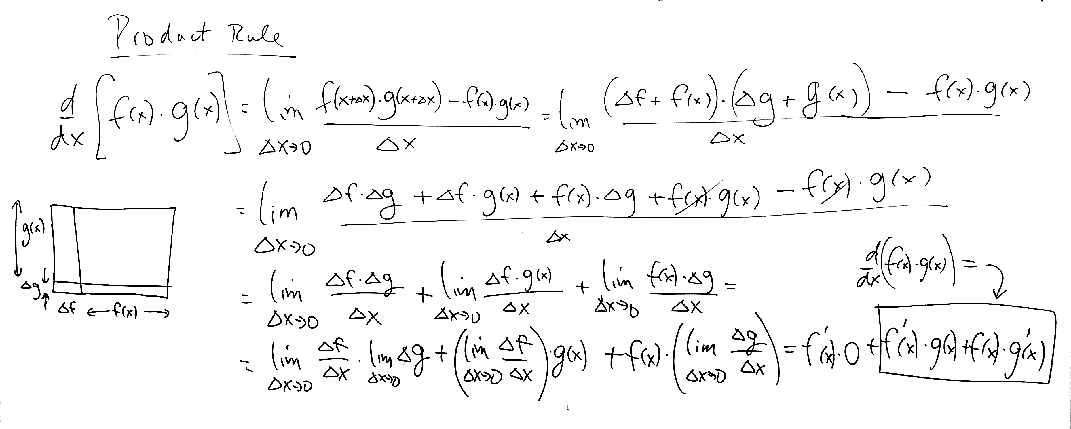
Here are proofs of the Product Rule and the Quotient Rule.
Worksheet on Derivative Shortcuts 3, with
the scanned solutions.
Wednesday, September 28: More on WeBWork set 9, start set 10
Rule:
\(\frac{d}{dx} [f(x)\cdot g(x)] =f'(x)\cdot g(x) + f(x) \cdot g'(x) \quad\) The product rule
Fact:
\(\frac{d}{dx} e^x = e^x \quad \) The derivative of the natural exponential function is itself!
Worksheet on Derivative Shortcuts 2, with
the scanned solutions.
Monday, September 26: The Derivative as a Function, WeBWork set 9
We start to learn how to differentiate any nice function.
Rules:
\(\frac{d}{dx} [c f(x)] = c f'(x) \quad\) The constant multiple rule
\(\frac{d}{dx} [f(x) \pm g(x)] = f'(x) \pm g'(x) \quad \) The sum and difference rules
Facts:
\(\frac{d}{dx} [c] = 0 \quad \) The derivative of a constant function is the 0 function
\(\frac{d}{dx} [x^c] = c x^{c-1} \quad \) The Power Function Fact (PFF)
Worksheet on Derivative Shortcuts 1, with
the scanned solutions
Monday, September 19: The definition of the derivative, WeBWork set 8
You will have 5 minutes to do Quiz 3. It will be given during the first 10 or 15 minutes of class. Here are
the scanned solutions and the
long version of the scanned solutions
An introduction to the derivative is motivated by this Quiz 3 follow up.
Definition: The derivative of the function \(f\) at \(a\) is the slope of the tangent line to \(y = f(x)\) at the point (\(a, f(a))\).
The notation for the derivative is \(f'(a)\), pronounced "\(f\) prime of \(a\)", and it can be computed as
\(\displaystyle f'(a) = \lim_{x \to a} \frac{f(x) - f(a)}{x-a}\).
Replace \(x\) with \(a + h\), so \(\Delta x = x -a = (a+h) - a = h\), and this becomes
\(\displaystyle f'(a) = \lim_{h \to 0} \frac{f(a+h) - f(a)}{h}\).
This is illustrated in this
Desmos graph.
Since \(a\) can be any point in the domain of \(f\), we can replace \(a\) by \(x\) and get our most useful way to compute the derivative.
\(\displaystyle f'(x) = \lim_{h \to 0} \frac{f(x+h) - f(x)}{h}\).
Given a function \(f\), this defines a new function, \(f'\).
Thursday and Friday, September 15 and 16: More Limits, WeBWorK set 7
Chapter 2 of
Paul's notes is a good resource for sets 1 through 7.
Worksheet 9, Limits at infinity,
with the
scanned solutions
Set 7 uses these two theorems, among other things:
The Squeeze Theorem:
Assume \(a < b < c\) and \(f_\ell(x) \leq f(x) \leq f_u(x)\)
for all \(x \in (a,b)\cup( b,c)\), and
\(\displaystyle \lim_{x \to b} f_\ell(x) = \lim_{x \to b} f_u(x) = L\).
Then \(\displaystyle \lim_{x \to b} f(x) = L\).
The Intermediate Value Theorem (IVT):
Suppose \(f(x)\) is continuous on \([a,b]\), and \(M\) is a number strictly between
\(f(a)\) and \(f(b)\). Then there exists a number \(c\) such that
\(a < c < b\), and \(f(c) = M\).
Wednesday, September 14: Continuity and Algebraic Limits, WeBWorK set 6
Here are some useful theorems that allow you to compute most of the limits you will encounter:
If \(f(x) = \tilde f(x)\) for all \(x \neq a\), and \(\tilde f\) is
continuous at \(a\), then \(\displaystyle \lim_{x \to a} f(x) = \displaystyle \lim_{x \to a} \tilde f(x) = \tilde f(a) \).
If \(f(x) = \tilde f(x)\) for all \(x > a\), and \(\tilde f\) is
continuous at \(a\), then \(\displaystyle \lim_{x \to a^+} f(x) = \lim_{x \to a^+} \tilde f(x) = \tilde f(a) \).
If \(f(x) = \tilde f(x)\) for all \(x < a\), and \(\tilde f\) is
continuous at \(a\), then \(\displaystyle \lim_{x \to a^-} f(x) = \lim_{x \to a^-} \tilde f(x) = \tilde f(a) \).
Worksheet 8, True/False questions about limits and continuity,
with the
scanned solutions
Here is the desmos graph of the
solution to my version of set 6, problem 12.
The function \(f\) is continuous if \(a = -1\) and \(b = -4\). You can use the sliders to see other versions of
Monday, September 12: Continuity and Algebraic Limits, WeBWorK set 6
Here are the Limit Laws,
and the definition of Continuity,
from Paul's notes.
Worksheet 7,
with the
scanned solutions
Friday, September 9: Graphical Limits, WeBWorK set 5
Definition of the Limit from 10:20 class whiteboard.
Worksheet 6 is in-class Quiz 2.
Here are the
scanned solutions
Thursday, September 8: Rates of Change, WebWorK set 4, and Graphical Limits, WeBWorK set 5
Worksheet 5 on
Slope of the tangent line.
Here are the
scanned solutions
and here is the link to the
desmos calculator solution.
Wednesday, September 7: Rates of Change, WebWorK set 4:
\(m_{PQ}\) is the slope of the secant line through points \(P\) and \(Q\) on the graph of a function.
Furthermore, \(m_{PQ}\) is the average rate of change of the function.
The slope of the tangent line at \(P\) is the limit of \(m_{PQ}\)
as \(Q\) approaches \(P\).
There is no posted worksheet today. In-class time is allowed for doing webwork
problems, especially problem 4.
Friday, September 2: Domain of Functions,
Composition of Functions, and Inverse Functions, WeBWorK set 3:
Worksheet 4 is in-class
Quiz 1, with
scanned solutions.
Thursday, September 1: Trig functions and
function notation, WeBWorK set 2:
In class worksheet 3 Domain of functions, and an application of Linear and Exponential Functions.
scanned solutions.
Wednesday, August 31: Linear and Exponential functions, WeBWorK set 1:
In class worksheet 2 on the Point-Slope Form for Linear Functions. scanned solutions.
Required knowledge from Precalculus
Instructor Information Jim Swift's home page Department of Mathematics NAU Home Page
e-mail: Jim.Swift@nau.edu