MAT 239 Schedule, Spring 2024

The links are to Paul's Notes, the section numbers refer to Boyce and DiPrima (10th edition).

WeBWorK set 1
Precalculus essentials
Differentiation essentials
Worksheet 1 is on paper and you will turn it in for attendance.
In class, we will go over WeBWorK problems 2, 3, 4, 5, 11, and 12. You can do this on your phone. It is a good idea to bring a tablet or laptop to class.

WeBWorK set 2
Introduction to WeBWorK, Classifying DEs. Definitions from Paul's notes (section 1.1, 1.2, 1.3 in Boyce and DiPrima).
direction fields (section 1.1)
Worksheet on Classification of DEs for the second day of class, with solutions.
Worksheet for the third day of class. Here are the scanned solutions to the first page of the worksheet.

WeBWorK set 3
Memorize these solutions and do NOT use separation of variables: Assume \(k\) and \(y_0\) are constants.
The general solution to \(\frac{dy}{dx} = ky\) is \(y = C e^{kx}\).
The solution to the IVP \(\frac{dy}{dx} = ky, \ y(0) = y_0\) is \(y = y_0 e^{kx}\).
separable 1st order ODEs (section 2.2)
Interval of Validity, or interval of existence, of solutions. (section 2.4)
Definitions of General Solution and Interval of Existence.
Worksheet 4 for the fourth day of class. Here are the scanned solutions.
We will have a quiz during the last 15 minutes of class.
Here are the scanned solutions of Friday's quiz.

WeBWorK set 4
Linear 1st order ODEs (section 2.1)
Recipe to solve any first order linear ODE for y(x). Here’s the recipe for y(t).
Worksheet 6. Here are the scanned solutions.
On Thursday, Feb. 1 we will start with Worksheet 7. Here are the scanned solutions.

WeBWorK set 5
1st order modeling (section 2.3). Solving dy/dt = k(y-A) by inspection.
Group work for Thursday, Feb. 1, worth 5 class points.
Here are the scanned solutions.
Worksheet on Modeling. Here is a compact version of the worksheet, for projection during class.
Here are the scanned solutions. Here is a full page solution to problem 3, taken from solutions to an old exam.

WeBWorK set 6
Autonomous Equations and Equilibrium Solutions (section 2.5). Euler's method (Section 2.7).
Worksheet 10. Here are the scanned solutions.
Here is a derivation of the solution to the logistic equation which is given to you in set 6, problem 5. Most textbooks do separation of variables, with partial fractions to do the \(P\) integral. Gross!

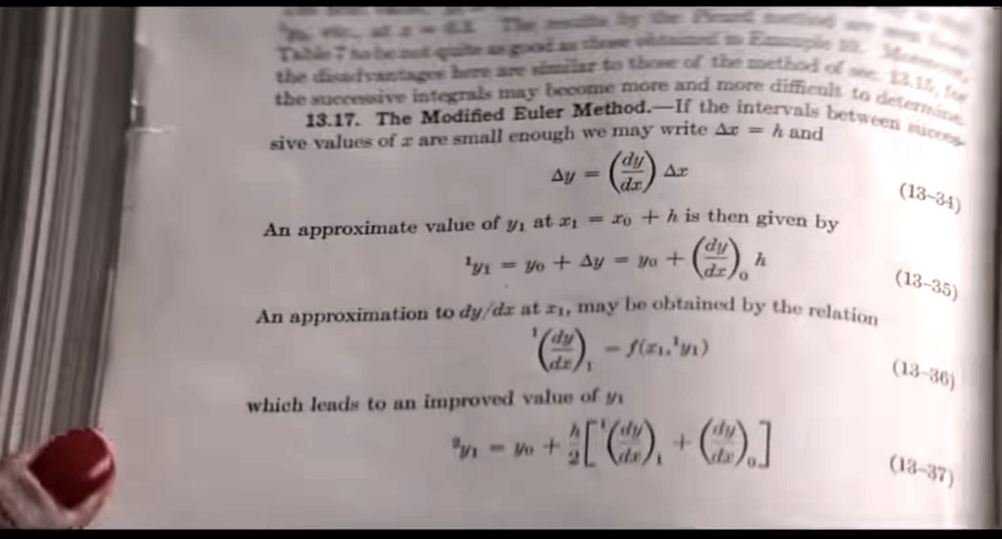
Euler’s method
Euler’s method scene from Hidden Figures.
I took this screen shot from the Hidden Figures Euler’s method Scene, with a descrption of the Modified Euler’s method. This method is also called Heun’s method, and it is the second method that our Slope Field and Direction Field applet uses. I found this desciption of the role math played in the Hidden Figures movie. This is a more nerdy blog about Katherine Johnson’s technical note which was mentioned in the film.

Here is a book chapter about Euler's Method, that you might prefer to Paul's notes on Euler's method (Section 2.7).
Here’s my pdf on how to do Euler’s Method with a Spreadsheet. We just do this together in class.
Here is my video on how to do Euler's Method with an Excel Spredsheet. (This video is not so good!)

WeBWorK set 7
Exact ODEs (Section 2.6).
These web sites might be helpful: CalcPlot3D, and Desmos Graphing Calculator.
Worksheet 12, on Exact ODEs. Here are the scanned solutions.
Tuesday, February 20: More about Exact ODEs, and Review for Thursday's exam
worksheet on solving exact ODEs. Here are the scanned solutions.

Exam 1 covering WebWorK sets 1-7 will be on Thursday, February 22. A sample exam is available on Canvas (in Assignments).
Here is the in-class review 1 worksheet. Here are the scanned solutions.

Thursday, February 22: Exam 1, covering WebWorK sets 1-7.
WeBWorK set 8 This is no longer assigned.

WeBWorK set 9
Basic Concepts and Real, Distinct Roots of the characteristic equation (sections 3.1, 3.2)
Worksheet 14. Here are the scanned solutions.
Here is a Desmos Graph of the general solution to \(y'' + y'-2y = 0\).
Find the solution to the IVP \(y'' + y'-2y = 0, \quad y(0) = 2, y'(0) = -1\) and check with this Desmos graph

WeBWorK set 10
Fundamental Solution Sets (Section 3.6), Linear independence, the Wronskian, and Abel's Theorem (section 3.7).
Problem 1 is about Linear Differential Operators, involving \(D = \frac{d}{dx}\) or \(D = \frac{d}{dt}\) depending on the context. Paul's notes do not talk about linear differential operators. We will use them extensively in this course. I suggest you check out these videos about Linear Differential Operators: Part 1 and Part 2.
Summary of the Theory of Linear Homogeneous ODEs.
Problems 4 is very much like Worksheet 16. Here are the scanned solutions.

For problem 5, use the Theory of Linear Homogeneous ODEs pdf, and these two facts about determinants:
(1): \(\text{det} \begin{bmatrix} a & b \\ c & d \end{bmatrix} = \text{det} \begin{bmatrix} a & c \\ b & d \end{bmatrix} = ad-bc\).
(2): Two vectors \( \langle a, b\rangle\) and \( \langle c, d\rangle\) are linearly independent if and only if \(\text{det} \begin{bmatrix} a & b \\ c & d \end{bmatrix} \neq 0\).
For problem 6, use Abel's theorem, which says that if \(y_1(t)\) and \(y_2(t)\) are any two solutions to \( y''+ p(t) y' + q(t) y = 0,\) then \( W_{y_1, y_2}(t) = c \ \text{exp}\left (-\int p(t) dt \right) \) for some constant \(c\).
The first order ODE version of Abel's theorem is that any solution to \(y' + p(t) y = 0\) satisfies \(y(t) = c \ \text{exp}\left (-\int p(t) dt \right) \) for some constant \(c\).

WeBWorK set 11
Complex roots of the characteristic equation, and Repeated roots of the characteristic equation. (section 3.3, 3.4, 4.1)
Euler equations (section 5.4).
Worksheet 17 for Tuesday, March 5 and Thursday, March 7. Here are the scanned solutions.
I make several videos to help with this problem set, and to justify the rules for solving Linear Homogeneous ODEs with Constant Coefficients (LHODECCs).
YouTube: Set 11, problem 1 (Solving \(y'' = k^2 y\) by inspection.)
YouTube: Set 11, problem 5 (A messy IVP)
YouTube: Multiple roots of the characteristic equation (Jusification of the rule)
YouTube: Complex conjugate roots of the characteristic equation (Jusification of the rule)
YouTube: Euler's Formula (Proof of \(e^{it} = \cos(t) + i \sin(t)\) using ODEs.)
YouTube: Hyperbolic Sine and Cosine functions that can be used to solve \(y'' = (\text{positive constant}) \cdot y\).
Desmos graphs of solutions to \(y'' = \text{constant} \cdot y\).
Taylor series of exp, cos, sin, etc.
Here is a pdf about how to solve \(y'' = \text{constant} \cdot y \ \) by inspection.

WeBWorK set 12
Linear nonhomogeneous ODEs (section 3.5, 4.3)
The Method of Undetermined Coefficients (included in sections 3.5, 4.3)
Worksheet 18 for Tuesday, March 19. Here are the scanned solutions.
Here is a pdf about the method of undetermined coefficients. Here are the solutions.
I made videos during the Spring 2020 lockdown for the rest of the class. The first set is here:
Set 12, Why is y = y_h + y_p?
Set 12, problem 5. Here is a link to the desmos graph for the solution to this problem.
Set 12, problem 8
Set 12, problem 10.
Set 12, problem 11

Here is a table from Boyce and DiPrima (10E) about how to choose the form of \(y_p = Y\).

WeBWorK set 13
Second Order Modeling, especially modeling of Mechanical vibrations (sections 3.7, 3.8)
Worksheet 21, Undamped Oscillators, for Tuesday, March 26. Here are the scanned solutions.
Videos
Set 13 introduction. Mass on a spring
Set 13, computing omega_0
Set 13, problem 1
Set 13, problem 2 introduction
Set 13, problem 2 finished
Set 13, problem 3
Set 13, problem 3 desmos . Here is the link to the desmos graph:
    polar coordinates for oscillators.
Set 13, damped oscillators
Set 13, damped oscillator graphs with Desmos graphing calculator . Here are links to the three desmos graphs discussed in the video:
    underdamped oscillator,
    overdamped oscillator, and
    critically damped oscillator.
Set 13, problem 6
Review: Second Order Modeling
NIST web page about the Quality Factor,Q
Desmos animation of a Shaken Mass on a Spring.
Desmos graph of the Resonance Curve, showing Full Width at Half Maximum Power.

Worksheet 23, Driven Oscillators, for Thursday, March 28. Here are the scanned solutions.

Worksheet 24, Exam Review, also for Thursday, March 28. Here are the scanned solutions.

Webwork set 13 is due Sunday, March 31, and
Exam 2 will be on sets 9-13, on Tuesday, April 2.

WeBWorK set 14
Review of Power Series and Taylor series (section 5.1 of Boyce and DiPrima).
Worksheet 25, Power Series Review, for Thursday, 04-04. Here are the scanned solutions.
Here's an animated gif of the Taylor Polynomials that approximate \(\displaystyle f(x) = \frac{1}{1+x^2}\). Note that \(T_5 = T_4\), and \(T_5\) is actually a polynomial of degree 4, not 5.
Videos
Set 14, problems 1-5
Set 14, problems 7 9 10
Set 14, problem 6
Set 14, problem 8

Second Worksheet for Thursday, April 4, on Taylor Series Review. Here are the scanned solutions.

WeBWorK set 15
Series Solution to 2nd order ODEs (sections 5.2 and 5.3 of Boyce and DiPrima).
Worksheet 26, Series Solution to \(y' +2y = 0\), for Tuesday, April 9. Here are the scanned solutions.
Videos
Set 15, problem 2
Set 15, problem 1
Set 15, solving recurrence relations This is useful for problems 2, 3, 4, and 5. Near the end the video shows how to do problem 4 (finding polynomial solutions with series methods) and gives a hint for problem 5 (getting an expression for \(c_{2n}\) or \(c_{2n+1}\) as a function of \(n\).)
Set 15, problem 6 sinc function
Set 15, problem 6
Set 15, more like problem 1

WeBWorK set 16
Systems of Linear Equations(not ODEs), Matrices and Vectors, Eigenvalues and Eigenvectors and Introduction to Systems of Linear ODEs (sections 7.1, 7.2 and 7.3 in Boyce and DiPrima).
Worksheet 27 on Systems of First Order ODEs, , for Tuesday, April 16. Here are the scanned solutions.
Videos
Set 16, Introduction to Systems of 1st Order ODEs, problems 1-4
Set 16, More about AB ≠ BA
Set 16, problems 5-7
Set 16, problems 8, 14 and 15 (Eigenvalues and Eigenvectors, part 1).
Set 16, Eigenvalues and Eigenvectors, Part 2 How to compute eigenvalues and eigenvectors.
Set 16, Eigenvalues example 1 (Real eigenvalues.)
Set 16, Eigenvalues example 2 (Complex eigenvalues.)
Set 16, Eigenvalues example 3 (Eigenvalues of a matrix with parameters.)
Here are figures of some vector fields and their eigenvalues and eigenvectors: eigenvalues 1 and 2, eigenvalues 1 and -2, irrational eigenvalues, pure imaginary eigenvalues, complex eigenvalues, repeated eigenvalues 0, 0, repeated eigenvalues -1.5, -1.5, and A = 2I with repeated eigenvalues 2, 2. Here is the Mathematica notebook, eigenvectors.nb, that made these figures.

WeBWorK set 17
Solutions to systems of Linear ODEs and the Phase Plane. Solutions to \({\bf x}' = A{\bf x}\), where \(A\) has Real Eigenvalues, Complex Eigenvalues and Repeated Eigenvalues (sections 7.5, 7.6, 7.8).

The solution to \(\bf x' = A \bf x\) , x(0) = x₀, for a \(2 \times 2\) matrix is fast and easy with the Swift method. Midterm 3 will give you these formulas.
A much longer paper describing this method is called Shortcuts for Solving Some Initial Value Problems. (This is only for the very curious!)

Worksheet 28 on Eigenvalues and Eigenvectors, for Thursday, April 18. Here are the scanned solutions.

Here are some other worksheets. We won't have time to do them all in class.
Finding a 2x2 matrix with a given pair of eigenvalues is easy with the eigenvalue hack described in this worksheet. Here are the scanned solutions.
Practice the Swift method with Worksheet 29.5. The solutions are the second page of the these scanned solutions.)
A worksheet on repeated eigenvalues and normal modes (like problem 10) is at Worksheet 30, with these scanned solutions.)
Videos
Set 17 intro to problems 1 to 9
Set 17 example 1 (Matrix has real, distinct eigenvalues.)
Set 17 example 1 computer pics
Set 17 problem 3, slow method (Complex eigenvalues, using the book's method)
Set 17 problem 3, swift method (Complex Eigenvalues, using the Swift method.)
Set 17 example 2 (problem 3) computer pics (WeBWorK problem 3 computer pics)
Set 17 example 3 (Matrix has repeated eigenvalues. Like WeBWorK problem 6.)
Set 17 examples 4 and 5 (Matrix has repeated, nonzero eigenvalues. Like WeBWorK problem 7.)
Set 17 examples 4 and 5 computer pics (Computer pictures for two matrices with repeated, nonzero eigenvalues.)
Set 17 problem 10 (Normal modes in a mass-spring system.)
Set 17 problem 10 computer animation

The Final Exam is scheduled for
Tuesday, May 7, 12:30-2:30, in our usual classroom.